Arduino + VL53L1X Time of Flight Distance Measurement
“As an Amazon Associates Program member, clicking on links may result in Maker Portal receiving a small commission that helps support future projects.”
Time of flight (ToF) is an approximation of the time it takes a traveling wave to come in contact with a surface and reflect back to the source. Time of flight has applications in automotive obstacle detection, resolving geographic surface composition, and computer vision and human gesture recognition. In the application here, the VL53L1X ToF sensor will be used to track the displacement of a ping pong ball falling down a tube. We can predict the acceleration and behavior of a falling ping pong ball by balancing the forces acting on the ball, and ultimately compare the theory to the actual displacement tracked by the time of flight sensor.
Time of flight uses the basic principles of Newtonian physics by assuming perfectly elastic contact with a surface. Most inexpensive ToF sensors use amplitude modulation to emit a singular or series of pulses at a particular frequency. For a laser, the frequency is usually in the infrared spectrum to ensure that the measurement is not visible to the human eye, and for an ultrasonic pulse its above the audible range. For an object at a distance x away from the light emitter (laser), we can approximate the reflection time for the light to hit the object and return back to the emitter:
where x is the distance to the object (2x because the signal has to reflect back), c is the speed of the wave (light here), and ΔT is the time it takes to travel 2x. This process is also shown in the image below.

The width of the signal pulse limits the minimum detectable distance and is often the working limit of the ToF module. This is a limitation of hardware that is capable of producing and reading short pulses of light. For example, a pulse width in the nano or pico second range are capable of resolving distances in the meter and millimeter ranges, respectively. The pulses are repeated hundreds or thousands of times to increase the sensor’s ability to measure longer distances. Therefore, the longer the desired distance, the longer the pulse ‘train’ needs to be. This means that either the pulses need to be shorter or the pulse train needs to be shorter to allow for longer reflections. More on ToF sensors and their limitations can be found here. The VL53L1X has a maximum range of 4m, which likely relates to a pulse width in the nanosecond range.
For this tutorial, I will be tracking the displacement of a ping pong ball falling down a tube using the VL53L1X time of flight sensor. The tube is used to both slow the ball down and also ensure the ToF sensor tracks the same position on the ball. An Arduino will be used to record the ToF measurements and a Raspberry Pi will be used to record and analyze the values. The full parts list is given below:
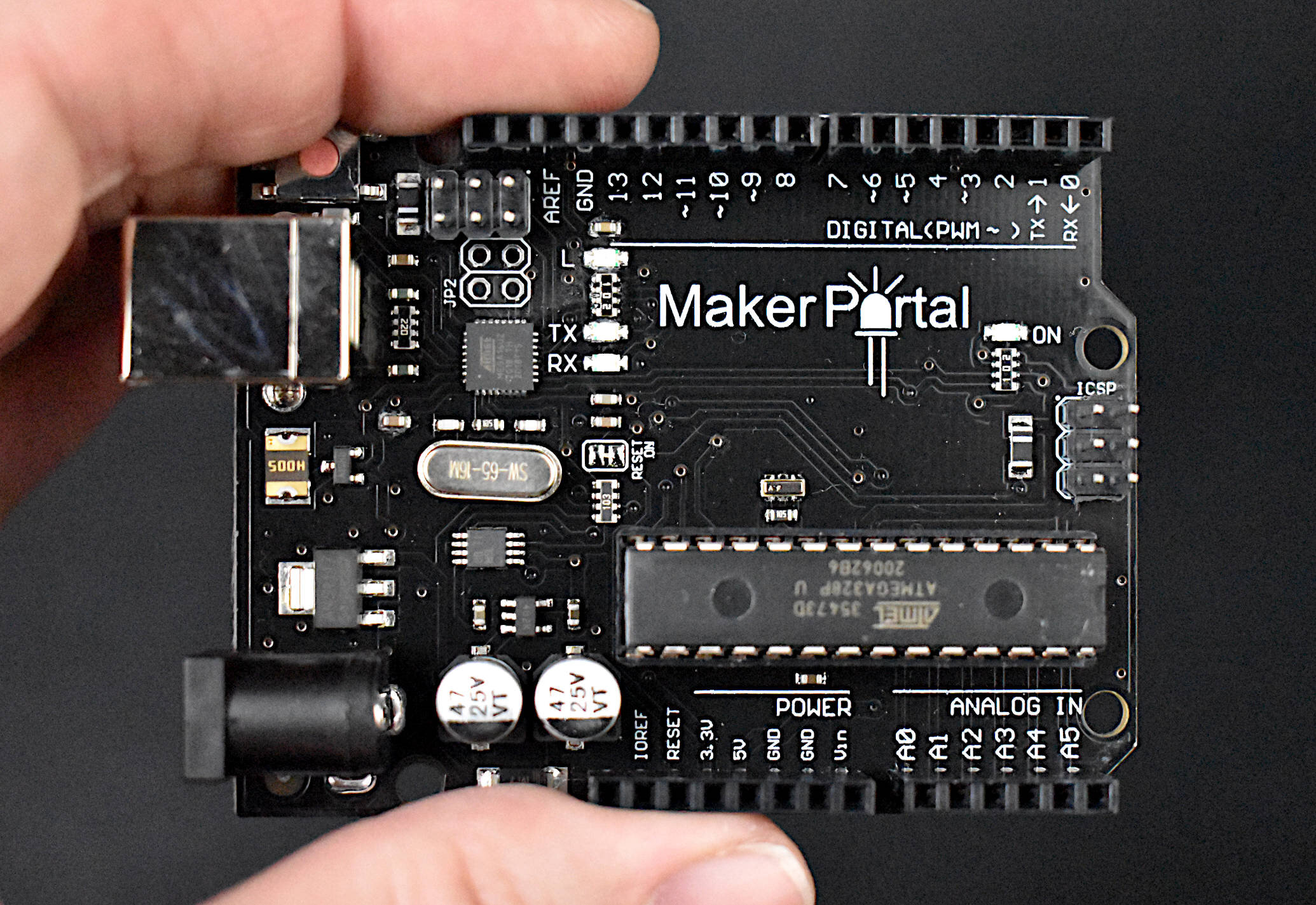
The Maker Portal Uno board is the centerpiece of many of the projects carried out in our maker spaces. The Uno board is capable of reading a wide range of sensors using analog-to-digital conversion, SPI, I2C, UART, and other common protocols. The Uno board can be used to control motors, OLED/LCD displays, and LEDs. The Arduino Uno board shown here is the official Maker Portal microcontroller, which we use in many of our projects!
Included in the Arduino Uno Package:
Maker Portal Arduino Uno Rev3 Board
Black USB Cable (1m in Length)
Specifications for Arduino Uno Rev3 Board:
ATmega328P chip with Arduino Bootloader
14 digital pins, 6 analog pins
10-bit analog-to-digital converter (ADC)
5V-12V Supply Tolerance
3.3V and 5.0V output pins
16 MHz clock
5 PWM pins, I2C support, SPI support , UART support
ATmega16U2 USB TTL, compatible with Linux, Windows, and Mac
Black Stylish Finish
Fully Integrated with Arduino IDE software
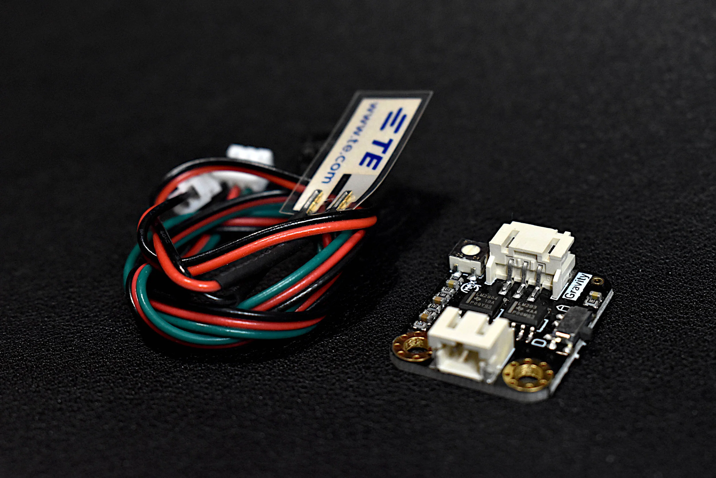
VL53L1X ToF Sensor - $21.99 [Amazon]
Ping Pong Ball - $6.17 [Amazon]
Acrylic Tube - $12.12 [Amazon]
Arduino Uno - $11.00 [Shop]
Raspberry Pi - $38.10 [Amazon]
Jumper Wires - $5.99 [Amazon]
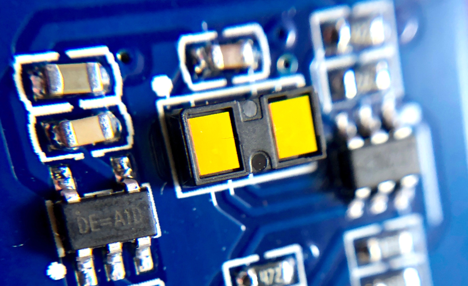
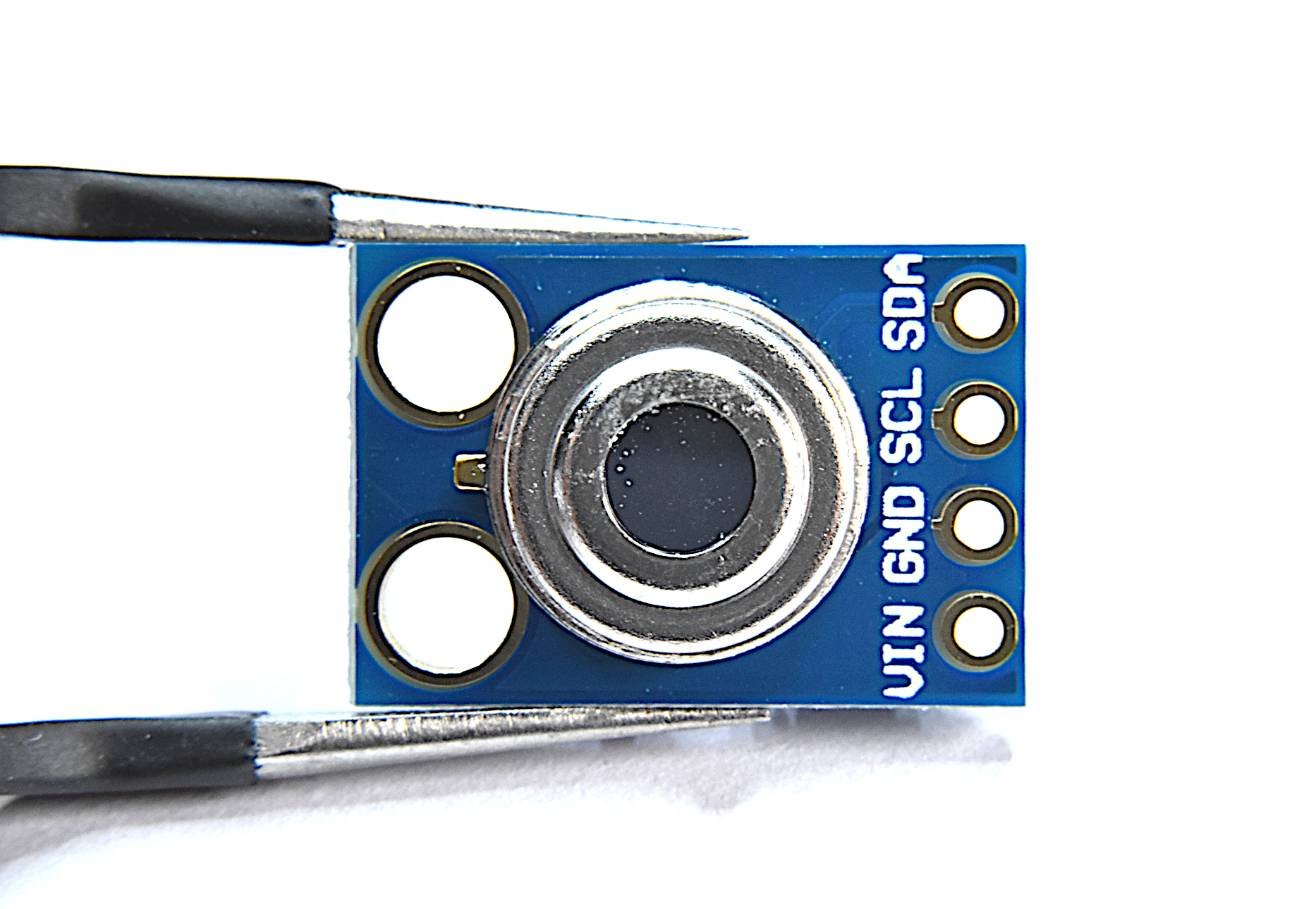
The VL53L1X can be wired to the Arduino board using the standard I2C ports on the Uno board (pins A4/A5). The wiring diagram is shown below:

In the next section, I will introduce the experimental setup for the ping pong ball falling down the tube and the VL53L1X placement in order to monitor the displacement of the falling ball.
For the actual experiment, the ball will be dropped by hand down the tube. The VL53L1X will be recording the time and displacement, which will then be read by the Raspberry Pi from the serial port. The setup of the ball, tube, and ToF sensor is shown below.

The basic setup for the experiment consists of a ping pong ball, VL53L1X sensor, and tube. The ball will be dropped from the top of the tube, and the VL53L1X will record the displacement of the ball as it travels down the tube due to gravity. The force balance for the ball is shown below:
The VL53L1X datasheet can be found here.

Force Balance on Falling Ping Pong Ball in a Tube
Applying Newton’s law leads to the following:
where Fg is the force due to gravity, FD is the drag force, and FB is the buoyant force. The equation above can be expanded and written in its explicit form:
where m is the mass of the ball, v is the velocity of the ball, g is the gravitation acceleration, ρf is the density of air, A is the aerodynamic area of the ball susceptible to drag, CD is the drga coefficient, and V is the volume of the ball. We can further rearrange the differential equation above and simplify a few parameters:
with the constants α and β defined as:
the differential equation has a solution of the form:
As an initial condition, we know the ball is not moving, so we can quantify the constant C0:
Therefore, our final velocity expression is:
Now, in order to approximate distance, we need to integrate the velocity:
which is much easier than the original differential equation, such that we now have an expression for the displacement as a function of time for a falling ping pong ball in a tube:
The VL53L1X library by Pololu is the simplest method for getting started with the ToF sensor. The code used to print the distance data from the VL53L1X is shown below.
#include <Wire.h>
#include <VL53L1X.h>

VL53L1X sensor;

void setup()
{
  Serial.begin(115200);
  Wire.begin();
  Wire.setClock(400000); // use 400 kHz I2C

  sensor.setTimeout(500);
  if (!sensor.init())
  {
    Serial.println("Failed to detect and initialize sensor!");
    while (1);
  }

  sensor.setDistanceMode(VL53L1X::Long);
  sensor.setMeasurementTimingBudget(15000);
  sensor.startContinuous(15);
  Serial.println("new program");
}

void loop()
{
  Serial.println(String(millis())+","+String(sensor.read()));
}
The code prints out milliseconds and distance for each measurement. The milliseconds prinout will allow us to attach a timestamp to each measurement. On the Raspberry Pi side, we can read the printout using Python’s Serial reader, pyserial. I wrote a full tutorial on reading from the serial port previously, which can be reviewed here. The code for reading the VL53L1X data is shown below:
import serial,time,csv,os
import numpy as np
import matplotlib.pyplot as plt

ser = serial.Serial('/dev/ttyACM0',
                    baudrate=115200)
ser.flush()
# overwrite file for saving data
datafile_name = 'test_data.csv'
if os.path.isfile(datafile_name):
    os.remove(datafile_name)
time_vec,dat_vec = [],[]
while True:
    try:
        ser_bytes = ser.readline()
        try:
            decoded_bytes = (ser_bytes[0:len(ser_bytes)-2].decode("utf-8")).split(',')
        except:
            continue
        if len(decoded_bytes)!=2 or decoded_bytes[0]=='' or decoded_bytes[1]=='':
            continue
        print(decoded_bytes)
        time_vec.append(float(decoded_bytes[0]))
        dat_vec.append(float(decoded_bytes[1]))

    except KeyboardInterrupt:
        print('Keyboard Interrupt')
        break
# plotting the data and saving points with the first points as the
# temporal and distance zeros
time_min = np.min(time_vec)
dat_min = np.min(dat_vec)
with open(datafile_name,'a') as f:
    writer = csv.writer(f,delimiter=',')
    for t,x in zip(time_vec,dat_vec):
        writer.writerow([t-time_min,x-dat_min])
plt.scatter(np.arange(0,len(dat_vec)),dat_vec)
plt.show()
The above code reads the Arduino data and saves it to two arrays (time and data). It also checks that the data is valid for temporal and distance formats and not invalid data. Then, once the user presses ‘CTRL+C’ the program stops and plots the data in terms of points. The points data should look like the figure below:

Raw Ball Drop Data Output in Python
The points shown here should be used to identify the start and finish points for the ball drop. The short jump around 60 is the ball hitting the ground and bouncing back toward the sensor. We do not want to include this in our calculation, which is why these start/end points are essential for processing.
In the next section, I address issues and results surrounding the ball drop experiment and the expectations when comparing the theory to experiments and how to properly handle the data and use the start/end points of the data shown in the figure above.
The assumption in this section is that the user was able to obtain data of the ball being dropped. The Python code should save the data shown in the profile above into a .csv file named ‘test_data.csv.’ Assuming all of this is true, the code and analysis to follow should be seamless. As stated in the theory sections above, we expect velocity and displacement profiles that follow those functions. We can now implement them into Python and see what the theory tells us about the expected behavior of the ball in the tube. The full code is shown below, but the pieces will be outline in a logical sequence that follows.
import csv
import numpy as np
import matplotlib.pyplot as plt

plt.style.use('ggplot')

# read data saved to csv file
with open('test_data.csv',newline='') as csvfile:
    reader = csv.reader(csvfile)
    data_vec,time_vec = [],[]
    for row in reader:
        time_vec.append(float(row[0])/1000.0)
        data_vec.append(float(row[1])/1000.0)

start_comp = 42 # point where ball is dropped
end_comp = 59 # point where ball hits ground
time_vec = np.subtract(time_vec[start_comp:end_comp],
                       time_vec[start_comp])
data_vec = np.subtract(data_vec[start_comp:end_comp],
                       data_vec[start_comp])

# functions for calcualting v and x analytically
def v_analyt_calc(t_i):
    return np.sqrt(beta_analyt/alpha_analyt)*np.tanh(np.sqrt(alpha_analyt*beta_analyt)*t_i)
def x_analyt_calc(t_i):
    return (1/alpha_analyt)*np.log(np.cosh(np.sqrt(alpha_analyt*beta_analyt)*t_i))

# aerodynamics and physical parameters
rho = 1.204 # density of air
m = 0.0027 # mass of ball
D_1 = 0.04 # diameter of ball
A_a = np.pi*(D_1/2.0)**2 # aerodynamic area of ball
C_D = 0.4 # drag coefficient of sphere
mu = 0.00001825 # dynamic viscosity of air
V = (4.0/3.0)*np.pi*np.power((D_1/2.0),3.0) # volume of sphere
rho_m = m/V # ball density
g = 9.8 # gravity

# differential eqn parameters
gamma = g*(1.0-((rho*V)/m))
beta_analyt = (1.0-(rho/rho_m))*g
C_D_analyt = 5 # effective drag coefficient
alpha_analyt = (1.0/2.0)*(rho/m)*A_a*C_D_analyt

# routine clarifications and allocations
dt = 0.001 # time step
t_range = np.arange(0,0.8,dt) # time vector for plotting
x_no_drag = ((g*(t_range**2))/2.0) # no drag, for comparison

# loop through time and calculate x and v
x_analyt,v_analyt,x_visc = [],[],[]
for t in range(0,len(t_range)):
    v_analyt.append(v_analyt_calc(t_range[t]))
    x_analyt.append(x_analyt_calc(t_range[t]))

# align theory and observation in time
t_match,x_dat_match,x_theory_match,v_theory_match = [],[],[],[]
for ii in range(0,len(time_vec)):
    t_diffs = np.abs(np.subtract(time_vec[ii],t_range))
    if np.min(t_diffs)>5*dt:
        continue
    match_loc = np.argmin(t_diffs)
    t_match.append(t_range[match_loc])

    x_theory_match.append(x_analyt[match_loc])
    x_dat_match.append(data_vec[ii])

    v_theory_match.append(v_analyt[match_loc])

# calculate mean absolute error between theory and observation
v_data_match = np.append(0.0,np.diff(x_dat_match)/np.diff(t_match))
mae = np.mean(np.abs(np.subtract(x_theory_match,x_dat_match)))
print('MAE (x): {0:2.5f} m'.format(mae))
v_mae = np.mean(np.abs(np.subtract(v_data_match,v_theory_match)))
print('MAE (v): {0:2.5f} m/s'.format(v_mae))

# plotting results
fig = plt.figure(figsize=(10,6))
ax1 = fig.add_subplot(2,1,1)
ax1.plot(t_range,x_no_drag,label='Theory, No Drag',linewidth=4)
ax1.plot(t_range,x_analyt,label='Theory, Analytical',linewidth=4)
ax1.plot(t_match,x_dat_match,label='Data',marker='.',linestyle='',
         markersize=15,color='#6fa664',markeredgecolor='k',markeredgewidth=0.5)
ax2 = fig.add_subplot(2,1,2)
ax2.plot(t_range,v_analyt,label='Theory',linewidth=4)
ax2.plot(t_match,v_data_match,label='Data',marker='.',markersize=15,linestyle='',
         markeredgecolor='k',markeredgewidth=0.5)
ax1.legend(fontsize=16,loc='upper left')
ax2.set_xlabel('Time [s]',fontsize=16)
ax1.set_ylabel('Displacement [m]',fontsize=16)
ax2.set_ylabel('Velocity [m/s]',fontsize=16)
ax2.legend(fontsize=16,loc='upper left')
ax1.axes.tick_params(axis='both',labelsize=12,pad=5)
ax2.axes.tick_params(axis='both',labelsize=12,pad=5)
ax1.annotate('Error: {0:2.0f}%'.format(100*(mae/np.mean(x_dat_match))),xy=(0.6,0.3),
             xycoords='data',xytext=(60,-5),size=14,textcoords='offset points')
ax2.annotate('Error: {0:2.0f}%'.format(100*(v_mae/np.mean(v_data_match))),xy=(0.6,0.3),
             xycoords='data',xytext=(60,-5),size=14,textcoords='offset points')
plt.show()
The three most important inputs in the code above are the ‘start_comp’ and ‘end_comp’ points and the drag coefficient ‘C_D_analyt.’ The start and end comparison points will determine where the effective ‘drop’ points are. Having the proper start and finish times are essential for proper comparison between theory and experiment, and it takes some manual work to find the true points. Second, the drag coefficient determines the speed at which the ball reaches terminal velocity, meaning that the higher the value for the drag coefficient, the quicker the ball will reach terminal velocity, the lower the drag coefficient, the longer it will take to reach terminal velocity. The terminal velocity for the ping pong ball, for example, can be seen to be about 2.4 m/s in the figure below.

If the start/end points were chosen correctly for the ball drop and the drag coefficient is appropriate (depending on the material of the tube and roughness of the ball), then the profiles should be similar to those above. A good way to determine if the endpoints are correct is to look at the time stamp - if the end time is around the time it takes the ball to hit the ground (something that can be measured with a stopwatch). Another way to verify the ending timestamp is to make sure the bounce after hitting the ground is not included. The bounce is easy to find because the velocity changes direction.
I found that a drag coefficient CD between 5-8 was fairly accurate for describing the behavior of the falling ping pong ball in an acrylic tube. If the tube manufacturing is inconsistent, or a different material on the ball or tube is used, this value will surely change. The same goes for a tube or ball of different diameter.
I also included the profile of a ball drop without any drag, which makes it easy to see just how essential it is that drag effects are included in the analysis of such an experiment.
The plot below is further validation that the experimental results are fairly accurate as well as repeatable. Five separate plots are given with the same drop experiment, but this time with a tube of 1.2 m length. We are not only proving our hypothesis, but also extending it by using a different sized tube. We can see that the ball profile reaches terminal velocity around the 0.5 second mark, where we start to see a linear displacement profile.

Surely, the theory and experiments do not match perfectly, there are neglected factors such as a non-constant drag coefficient, however, for the purposes of this experiment we are still able to recover theoretical displacement results within 9% of the experimental values.
The VL53L1X time of flight sensor is a powerful sensor that is capable of resolving fast changes in distance with fairly accurate and consistent results. This experiment proved the reliability of a ToF sensor for approximating displacement of a moving object. The relatively high sample rate (20Hz-50Hz) of the VL53L1X was able to resolve the quick movements of a ping pong ball down an acrylic tube, which allowed us to compare the theoretical displacement prediction to the actual physical behavior of the ball. The experiment can be used as an educational tool for fluid mechanics classes and engineering students to explain the viscous effects of pipes and surface area drag effects. We were able to determine an approximate drag coefficient for the system, around 6, which could be used to characterize a similar system involving traveling objects in tubes. Lastly, the real-world example demonstrates an end-to-end experimental and theoretical development of a physical system - something that could be useful to students and professionals interested in studying fluid mechanics and experimentation in engineering.
Social Links
Related Tutorials


See More in Engineering: