Raspberry Pi Vibration Analysis Experiment With a Free-Free Bar
For engineers, vibration analysis is key for both understanding and predicting behavior in complex structures and processes. Vibrating structures can include bridges, buildings, and aircraft - all of which require extensive research and understanding in order to ensure reliable and safe construction. In this tutorial, beam vibrations will be measured to demonstrate a real-world example of a vibrating sturcture. The study of beams is important because they are inherently susceptible to vibration due to their long and thin construction and high stress applications, such as aircraft wings or bridge supports.
Using the Euler-Bernoulli beam theory, the resonant frequencies of a beam will be measured using a thin film piezoelectric transducer and compared to the theoretical calculations. A Raspberry Pi will be used along with a high-frequency data acquisition system (Behringer UCA202, sample rate: 44.1kHz) and the Python programming language for analysis. The fast fourier transform will allow us to translate the subtle beam deflections into meaningful frequency content. This tutorial is meant to introduce Python and Raspberry Pi as formidable tools for vibration analysis by using measurements as validation against theory.

The Euler-Bernoulli beam theory is an application of linear beam theory that relates the forces experienced by a beam to the deflection of the beam. We can investigate the behavior of a vibrating beam by analyzing the forces on an incremental portion:
Using the above setup we can derive the relationship for beam deflection as a function of location along the beam and time. This relationship is of the following form [resources on derivation: Vibration of Continuous Systems, Transverse Vibration Analysis of Euler-Bernoulli Beams Using Analytical Approximate Techniques, Vibration of Continuous Systems, Transverse Waves in Rods and Beams]:
The general solution to the equation above can be found using separation of variables:
The full derivation of the general solution can be downloaded here.
We now can establish boundary conditions such that we can find the natural modes of the beam and setup theoretical values to compare against our experiments later in this tutorial. We will be using a free-free beam, which means the beam is not clamped or fixed at either side. The boundary conditions for this condition are:
Solving the general solutions to the differential equation for the boundary conditions above leads to the following transcendental solution for the natural modes of the beam:
Which we can solve using a numerical method. I attached a Python code which approximates the locations where the equation is valid, and plotted the zero locations found by the algorithm below. The first ten non-zero roots are shown on the plot below. Beyond this range, it is my belief that the computer program has trouble resolving rounding issues with the logarithm in the cosh() function above, resulting in larger error. The first seven modes below, however, have errors less than 0.0003 in their zero approximation of the root.
## Calculating the zeros of transcendental equation
#
import numpy as np

# function for calculating specific transcendental equation
def trans_calc(x):
    return np.cosh(x)*np.cos(x)-1.0

max_root = 35.0
num_iterations = 10000.0
gamma_L_vector = np.linspace(0.0,max_root,num_iterations) # vector for looping values
y = trans_calc(gamma_L_vector) # first iteration of solving
diff_vec = np.divide(np.append(0,np.diff(y)),y) # loop at difference (similar to derivative)

deriv_peak = 1.0
zero_vals = [gamma_L_vector[i] for i,x in enumerate(diff_vec) if x>deriv_peak] # approx. zero values
zero_locs = [i for i,x in enumerate(diff_vec) if x>deriv_peak] # locations of approx zeros

# loop for better approximation of zeros
gamma_L_array,trans_val_array = [],[]
max_loops = 1000
num_iterations = 1000.0
for ii in range(0,len(zero_vals)):
    loop_num = 0
    gamma_L_new = np.linspace(gamma_L_vector[zero_locs[ii]-1],gamma_L_vector[zero_locs[ii]+1],num_iterations)
    y_new = trans_calc(gamma_L_new)
    zero_vals_new = gamma_L_new[np.argmin(np.abs(y_new))]
    zero_locs_new = np.argmin(np.abs(y_new))
    while np.abs(trans_calc(zero_vals_new))>0.0:
        gamma_L_new = np.linspace(gamma_L_new[zero_locs_new-1],gamma_L_new[zero_locs_new+1],num_iterations)
        y_new = trans_calc(gamma_L_new)
        zero_locs_new = np.argmin(np.abs(y_new))
        zero_vals_new = gamma_L_new[np.argmin(np.abs(y_new))]
        if loop_num<max_loops:
            loop_num+=1
        else:
            break

    # print out new approximations and the values near zero
    print('Root: {0:2.5f}'.format(zero_vals_new))
    print('Value: {0:2.5f}'.format(trans_calc(zero_vals_new)))
    print('-------------')
    gamma_L_array.append(zero_vals_new)
    trans_val_array.append(trans_calc(zero_vals_new))
The first eight zero-crossings for the modes of a free-free beam are:
| 0 | 0 |
| 1 | 4.730040744862704 |
| 2 | 7.853204624095838 |
| 3 | 10.995607838001671 |
| 4 | 14.137165491257464 |
| 5 | 17.27875965739948 |
| 6 | 20.42035224562606 |
| 7 | 23.561944902040455 |
| 8 | 26.703537555508188 |
Now that we’ve solved the transcendental equation, we can look to solve the general solution to the beam equation for our specific boundary conditions. The specific solution for a free-free beam is a combination of the two temporal and spatial components mentioned above. The complete solution is:
The first modal frequency is shown below (calculated using the particular solution, the numerical solution to the transcendental equation, and the specific equation for frequency from our geometry). I used: D = 0.008 m, ρ = 7800, E = 200 GPa, and L = 0.5 m.

The first four modes of the vibrating bar (defined down to 0.1 Hz -> the max resolution of the acquisition sampling) will be compared with the actual measurements of a bar in the experiment to follow.
n = 1, f = 144.3 Hz
n = 2, f = 397.6 Hz
n = 3, f = 779.5 Hz
n = 4, f = 1288.6 Hz
This experiment will explore the free vibrations of a cylindrical beam by measuring the natural vibration frequencies of the beam. This will be done by attaching a piezoelectric sensor to the end of the beam and measuring the deflection changes over time (using the data acquisition system and the Raspberry Pi). This will allow us to approximate the deflection frequencies using Python by analyzing the FFT of the resulting time-series signal. The four main parts used in the experiment are listed below, as well as links to other parts relevant to the project:
Steel Rod (8 mm x 406 mm) - $8.99 [Amazon]
Piezo Vibration Sensor - $15.00 [Our Store]
Raspberry Pi 3B+ - $38.50 [Amazon]
Behringer UCA202 USB Interface - $29.99 [Amazon]
“As an Amazon Associates Program member, clicking on links may result in Maker Portal receiving a small commission that helps support future projects.”
Wiring for Vibration Analysis Using Raspberry Pi and The Behringer UCA202
The voltage divider is necessary for lowering the output signal from the piezo sensor to 1.5 V (from 5V), which is the max input for the Behringer UCA202. The Behringer UCA202 samples the piezo vibrations at 44.1 kHz (or 48.0 kHz), and the piezo film measures small deflections from the vibrating bar. This is the simple setup for the vibration analysis of the bar using the piezo element and the RPi. In the next section, the measurement methods will be introduced as well as some Python routines for acquisition and analysis.
A free-free bar should be suspended without interference when measuring its natural modes, however, this is impossible. The simple way of avoiding interference is to support the bar at specific mode nodes. For example, we can use the solution for the vibrating bar at particular modes and find the locations that have no deflection.
The image shown here shows the piezo sensor fixed to the edge of the steel cylindrical bar. This method enables the piezo film to measure the quick deflections taking place at the end of the bar due to induced vibrations.

Piezo sensor fixed atop the cylindrical bar
Experimental Procedure
- Identify the natural modes of the bar using a numerical method and approximate each mode’s support location
- Support the bar at each respective mode node
- Attach the piezo film at one end of the bar
- Prepare the data acquisition by recording background noise
- Strike the bar with a rubber tool
- Record the vibrations and analyze the frequency spectrum of the resulting oscillations
I found that the best method for exciting the bar is to strike it with a rubber mallet or handle. I used the rubber handle of a screwdriver - but a mallet would be optimal to avoid any high-frequency elastic or inelastic contact between the bar and striking tool, which could cause unwanted behavior of the bar. Below is a slow motion clip where the bar is struck by the rubber handle, after which the bar vibration can both be seen and heard:
We can identify the zero locations and approximate them, which I have done in the animation below:

This animation agrees with the literature and other similar studies done on free-free beams. A great example of the free-free beam modes can be found on the popular: hyperphysics.phy-astr.gsu.edu website, where they state the same zero-locations found for the n = 1 case.
| |
||
|---|---|---|
| 144.3 | 0.22416 | 0.77584 |
| 397.6 | 0.13211 | 0.86789 |
| 779.5 | 0.35580 | 0.64420 |
| 1288.6 | 0.27678 | 0.72322 |
Below is the Python code used to calculate the bar vibration frequencies measured by the piezo element:
import pyaudio
import matplotlib.pyplot as plt
import numpy as np
import time

plt.style.use('ggplot')

def fft_calc(data_vec):
    fft_data_raw = (np.fft.fft(data_vec))
    fft_data = (fft_data_raw[0:int(np.floor(len(data_vec)/2))])/len(data_vec)
    fft_data[1:] = 2*fft_data[1:]
    return fft_data

# using the Behringer UCA202 as an audio acquisition system at 44.1kHz and 16-bit
form_1 = pyaudio.paInt16 # 16-bit resolution
chans = 1 # 1 channel
samp_rate = 44100 # 44.1kHz sampling rate
chunk = 44100*10 # 2^12 samples for buffer
rec_secs = 10
dev_index = 2 # device index found by p.get_device_info_by_index(ii)

audio = pyaudio.PyAudio() # create pyaudio instantiation

# create pyaudio stream
stream = audio.open(format = form_1,rate = samp_rate,channels = chans, \
                    input_device_index = dev_index,input = True, \
                    frames_per_buffer=chunk)
stream.stop_stream()
# record background noise
input('press enter to record noise')
stream.start_stream()
noise = np.fromstring(stream.read(chunk),dtype=np.int16)
stream.stop_stream()

fft_noise =fft_calc(noise) # fft of noise

# record the actual bar vibrations
input('press to record actual data')
stream.start_stream()
data = []
for ii in range(0,int(np.floor((rec_secs*samp_rate)/chunk))):
    data.extend(np.fromstring(stream.read(chunk),dtype=np.int16))
stream.stop_stream()
print('finished recording')

# prepare plots
fig = plt.figure(figsize=(10,6))
ax = fig.add_subplot(2,1,1)
t_vec = np.linspace(0,len(data)-1,len(data))*(1/samp_rate)
ax.plot(t_vec,data,label='Time Series')

f_vec = samp_rate*np.arange(chunk/2)/chunk # fft frequency vector
fft_vec = []

# here we're subtracting the noise from the actual data FFT
for jj in range(0,int(np.floor((rec_secs*samp_rate)/chunk))):
    fft_vec.append(np.abs(fft_calc(data[jj*chunk:(jj+1)*chunk]))-np.abs(fft_noise))

fft_data = np.mean((fft_vec),0) # if there's more than 1 sample period, average the FFTs

freq_range = (100.0,20000.0) # frequency range set above the noise of the piezo element

min_locs = (np.argmin(np.abs(np.subtract(f_vec,freq_range[0]))),
            np.argmin(np.abs(np.subtract(f_vec,freq_range[1]))))
f_plot = f_vec[min_locs[0]:min_locs[1]] # frequencies to plot
y_plot = (fft_data[min_locs[0]:min_locs[1]]) # data to plot

# plot setup
plt.xlabel('Time [s]')
plt.ylabel('Amplitude')
plt.legend()

ax2 = fig.add_subplot(2,1,2)
ax2.plot(f_plot,y_plot,label='Freq Spectrum')
ax2.set_xscale('log')
##ax2.set_yscale('log') # can use the log y-scale if the data amplitudes are small
ax2.set_ylim([0.1,3.0*np.nanmax(y_plot)])
ax2.set_xlim([freq_range[0],freq_range[1]])

plt.xlabel('Frequency [Hz]')
plt.ylabel('Amplitude')
plt.legend()

# annotate the max values around the approximate frequencies calcualted in the theoretical section
annot_y_max = 2.0*np.max(y_plot)
freq_theory_array = [145,400,784,1297] # theoretical frequencies
search_width = 30.0 # max width to look for frequencies around the theory
for mm in range(0,len(freq_theory_array)):
    freq_range = (freq_theory_array[mm]-search_width,freq_theory_array[mm]+search_width)
    min_locs = (np.argmin(np.abs(np.subtract(f_vec,freq_range[0]))),
            np.argmin(np.abs(np.subtract(f_vec,freq_range[1]))))
    f_plot = f_vec[min_locs[0]:min_locs[1]]
    y_plot = (fft_data[min_locs[0]:min_locs[1]])
    print('f_max = {0:2.1f}'.format(f_plot[np.argmax(y_plot)]))
    ax2.annotate('{0:2.1f}'.format(f_plot[np.argmax(y_plot)]),
                xy=(f_plot[np.argmax(y_plot)],np.max(y_plot)),
                xytext=(f_plot[np.argmax(y_plot)],annot_y_max),
                arrowprops=dict(facecolor='k',shrink=0.05),
                horizontalalignment='center',
                fontsize=14,
                )
plt.tight_layout()
plt.savefig('bar_natural_resonance_FFT.png',dpi=300,facecolor=np.array([252,252,252])/255.0) # save the figure
plt.show()
In the next section, the theoretical frequencies will be compared to the values measured at the support locations outlined in the table above.

Project Sponsor: PCBGOGO.COM
Below is a series of four plots, each containing data sampled at 44.1 kHz for 10 seconds (resulting in a frequency resolution of 0.1 Hz). Both the time series and FFT of the signal are displayed. For each support location, the frequencies pertaining to the particular location is indicated by an arrow and were used as the measured value for each respective support location.
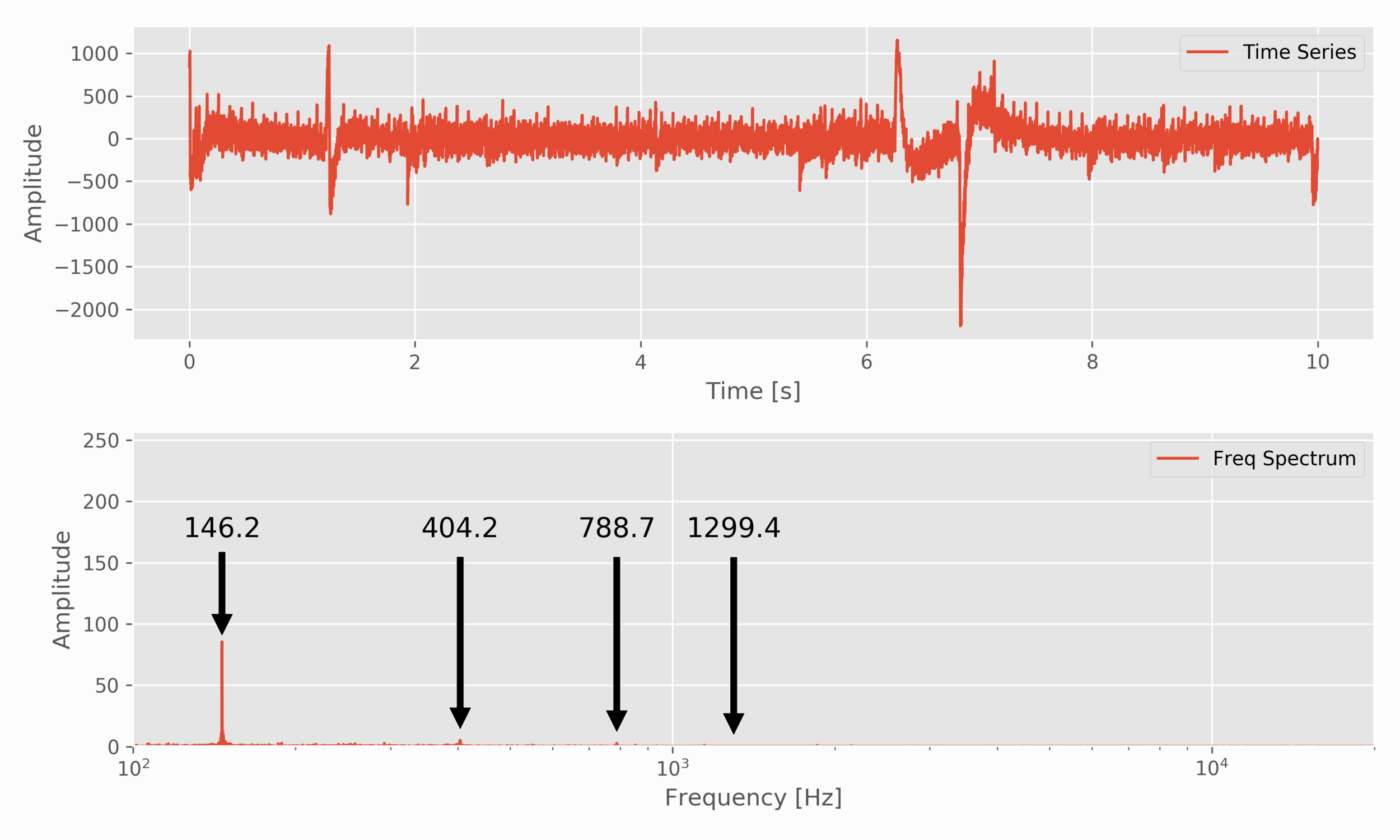
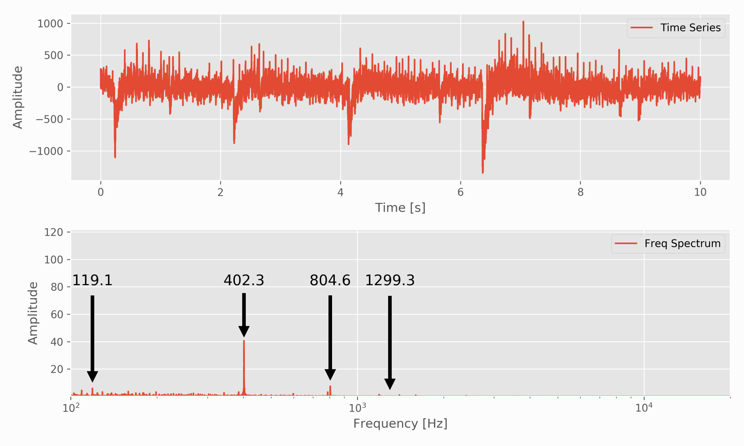
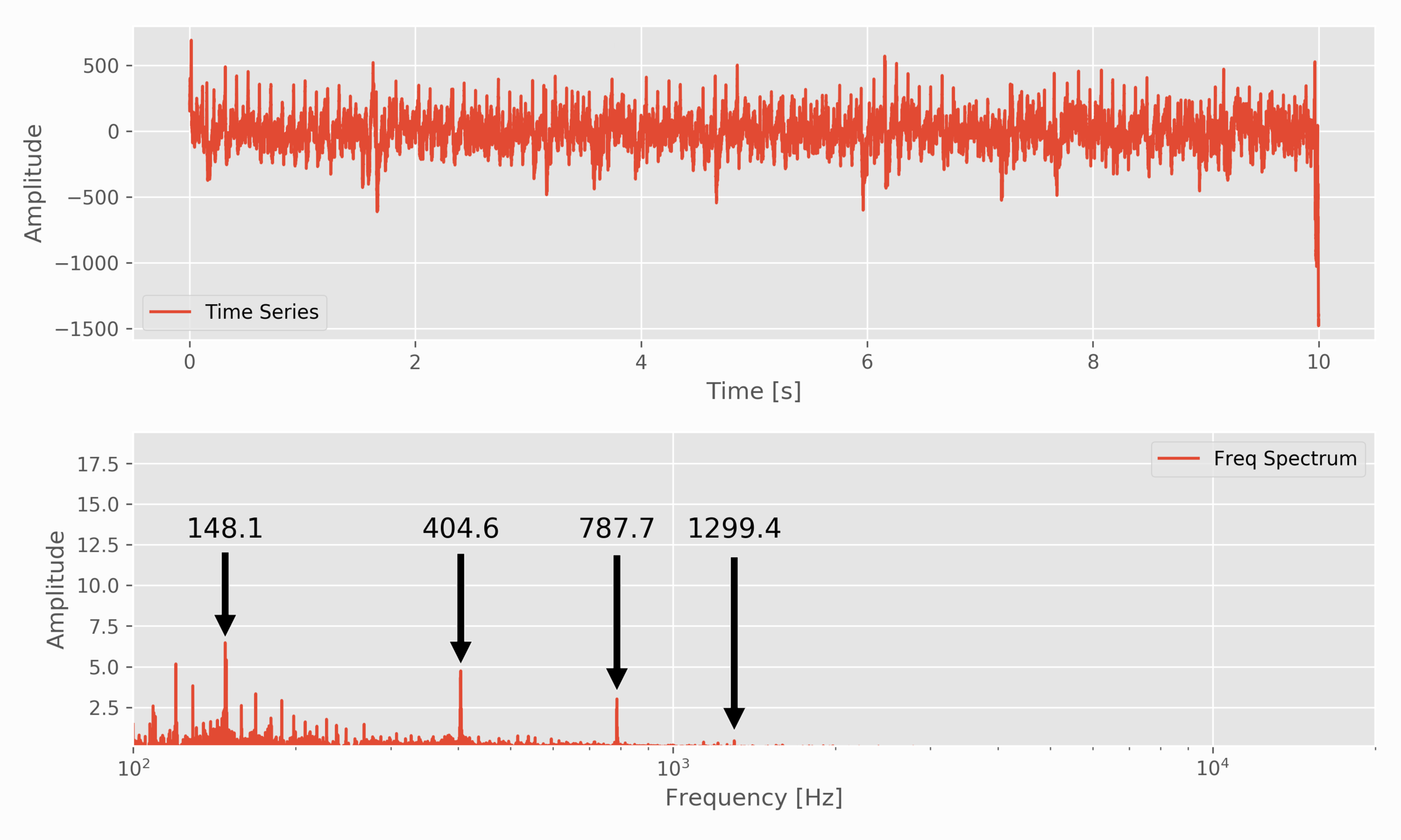
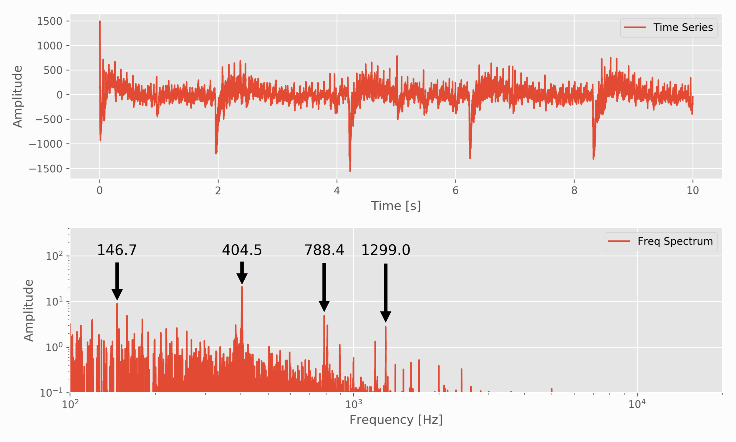
The measured frequencies were recorded as follows:
146.2 Hz
402.2 Hz
787.7 Hz
1299.0 Hz
It may or may be obvious that the values are consistently higher than the theoretical calculations. This could be a result of a multitude of errors in machining of the bar, approximation of the elastic modulus, errors in the measurement method - it’s hard to say. However, one hypothesis we can at least attempt to correct is the elastic modulus.
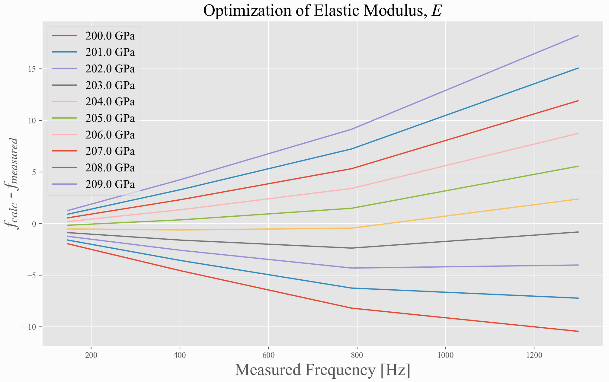
Iterating Over Nearby Elastic Moduli to Find the Best Frequency Fit
Optimal E = 204.2 GPa
| 145.8 | 146.2 | 0.27 |
| 401.8 | 402.2 | 0.10 |
| 787.6 | 787.7 | 0.01 |
| 1302.0 | 1299.0 | 0.23 |
The results demonstrate that if the proper support locations are used for measuring specific frequencies, the error between theory and measurement can be approximated within 1%. This also suggests that the resonant method using a piezo element is a viable option for approximating Young’s modulus (elastic modulus) for different materials.
This experiment has demonstrated several theories in engineering. The first: the Raspberry Pi is capable of handling a robust vibration analysis - something that is impressive considering the traditional requirements for conducting such an experiment. Second, the closeness of theory and experiment indicates that our assumptions are correct and the measurement methods are also accurate and acceptable. This builds confidence in the user’s ability to conduct similar experiments on new materials with unknown properties - something that may be useful in industry.
The goal of this tutorial and experiment was to endow the user with a sense of real-world parallel to a complex engineering problem. The principles employed here utilize skills in solid mechanics, partial differential equations, experimental analysis, and data analysis - all of which are useful to an engineer. Another intention of the experiment was to demonstrate the capabilities of the Raspberry Pi and conquer a difficult, real-world problem that is able to be solved with inexpensive and open-source tools.

See More in Engineering and Data Analysis: