Solar Panel Characterization and Experiments with Arduino

“As an Amazon Associates Program member, clicking on links may result in Maker Portal receiving a small commission that helps support future projects.”
Photovoltaic cells, commonly referred to as PV cells, are at the center of all solar panels and are responsible for the conversion of solar energy into electricity. The study and theory of photovoltaic power production is quite complex and involves understanding the non-linear relationship between voltage (V) and current (I), which is generated by solar insolation and impacted by the electronics present in a given panel configuration [read more about PV cells and solar arrays here and here]. In this tutorial, the aim is to characterize a solar panel by varying the load at (near) peak solar insolation to identify the panel's nominal values such as open-circuit voltage, short-circuit current, max power voltage and current, and max power output. These values help users understand the expectations from a photovoltaic array and how their power needs may be met with a given PV system. An Arduino board will be used to log the current and voltage values outputted from a small solar panel. The current and voltage are measured using a 16-bit analog-to-digital converter power module, the INA226, which will allow us to track the power outputted from the photovoltaic panel. A potentiometer acting as a rheostat will serve as the varying load on the system, which will be used to identify the peak power points of the system. Finally, analyses will be conducted in Python 3, which will allow us to identify the peak power region and also the total power outputted over a duration of 24 hours.
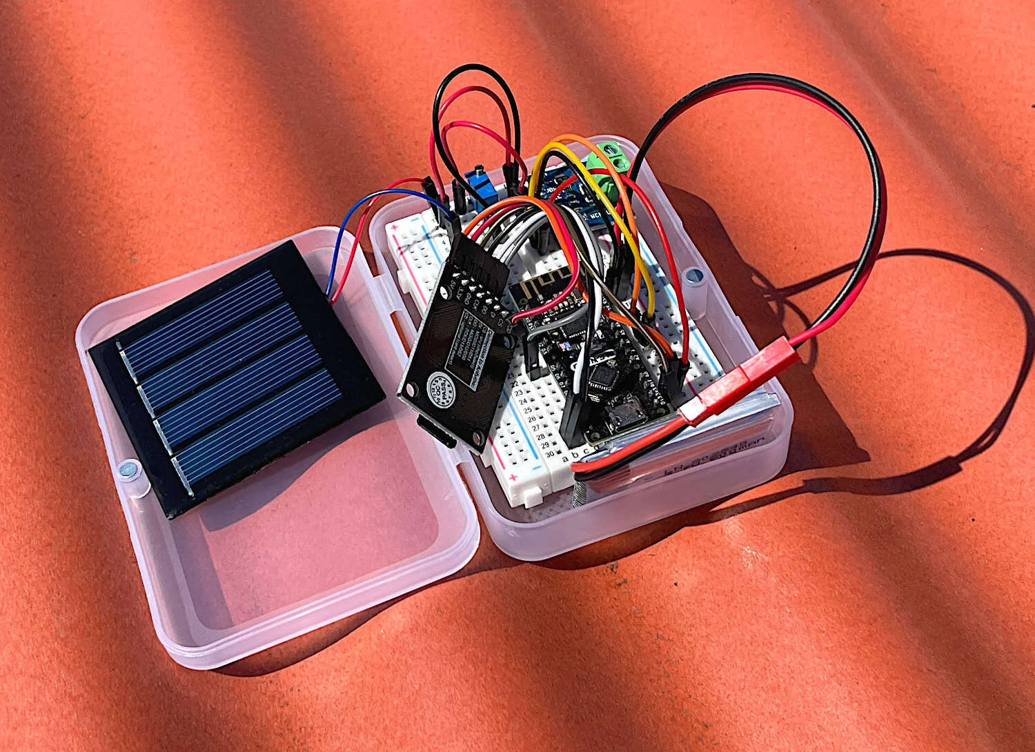
There are many components used in this project, ranging from the solar panel itself to the voltage/current sensor (INA226) and SD module. The full parts list is given below, for reference. We have also developed a kit that contains the most important components used in the project, though all parts can be sourced individually either from our shop or elsewhere.
Parts List:
Solar Panel (limited to 0.5W for rheostat) - $7.00 [Our Store]
INA226 Current/Voltage Sensor - $6.00 [Our Store]
BLE-Nano Board - $15.00 [Our Store], $22.00 (MakerBLE alternate)
SD Card Module - $8.00 [Our Store]
16GB SD Card - $10.00 [Our Store]
1kΩ Potentiometer - $11.99 (60pcs Kit) [Amazon]
LiPo Battery, 3.7V 600mAh - $15.00 [Our Store]
Electronics Component Box - $3.00 [Our Store]
Large Breadboard (400 Ties) - $6.00 [Our Store]
Jumper Wires - $3.00 (10x Male-to-Male, 10x Female-to-Male) [Our Store]

This kit is geared toward engineers and makers interested in learning about solar energy and how to characterize solar cells, understand nominal values in solar technology, and how to collect meaningful data. The kit comes with a solar panel, SD card and module for datalogging, a potentiometer, and LiPo battery for portability. The user just needs to add an Arduino board and breadboard and they can start logging solar data and make calculations in their local environment.
Included in the Solar Panel Datalogger Kit:
1x 2V, 120mA Solar Panel (54mm x 54mm) [Wire Colors May Vary]
1x INA226 Voltage/Current Measurement Module
1x 1kΩ Potentiometer (Rheostat in Experiments)
1x 3.7V, 600mAh LiPo Battery + USB Charger
1x SD Datalogger Module
1x 16GB SD Card
10pcs Female-to-Male + 10pcs Male-to-Male Jumper Wires
Features of the Solar Panel Datalogger Kit:
Characterize Solar Panel by Varying 1kΩ Potentiometer
600mAh Battery Allows for Roughly 1 Day+ of Datalogging (Depending on the Arduino Board and Sleep Routines)
16GB SD Card + Module Allow for Long-Term Datalogging
INA226 Reads 16-bit Voltage and Current
54mm x 54mm Solar Panel has 4 cells each 10mm x 38mm, for an Active Area of 15.2 cm-sq
See our tutorial on using the kit: Solar Panel Characterization and Experiments with Arduino
The wiring diagram for the collective system is given below:

Note: we have omitted any explanation of the wiring configuration in order to declutter the tutorial, however, most of the wiring explanations can be found either on our site or in other literature/forums online. We will discuss the solar panel, potentiometer (rheostat), and INA226 current/voltage configuration later in the experimental setup section. The rest are left for the user to explore.
Solar panels often consist of an array of photovoltaic cells arranged in a way that produces a desired power output at a given voltage and current configuration. This allows users and operators to select the load based on the desired output or the panel based on the load requirement. This is why the characterization of solar panels and PV cells is of utmost importance, for both the assurance of power generation and safety of operation. That being said, sometimes it is more advantageous to model solar panels rather than develop them and characterize them later. Unfortunately, PV array models are complex and involve many co-dependent components, all of which impact the behavior, and thus the output, of the solar panel. The simplest model for a PV cell can be written as the relationship between voltage and current, as follows:
If we were to plot this relationship, we would get the following profile:

Basic Solar Cell Voltage/Current Profile
Expected output before any electrical components are added to the solar cell system.
This is the simplest representation for a solar cell. Notice that there are no numbers on the plot - this is due to the fact that we need to know a bit more about the system before we attach any real-world values to anything.
For any practical application, the solar measurement will include some electrical components which will affect the profile shown in the figure above. Thus, in most models of PV cell power output involve at least shunt and series resistors. The resulting equivalent circuit is as follows:

- E0 ≡ Solar Insolation
- IL ≡ Photogenerated current
- ID ≡ Diode current
- ISH ≡ Shunt current
- RSH ≡ Shunt Resistance
- RS ≡ Series Resistance
- V ≡ Cell Voltage
- I ≡ Cell Current
If we were to setup the equation that solves for current as a function of voltage using the circuit above, we arrive at the common and applicable PV expression:
And here we have a more complex and difficult to solve implicit equation that relates parameters of the system to the power output potential of the cell (voltage multiplied by current). There are numerous references that have parametrically solved or empirically solved for voltage as a function of current and vice-versa, however, that is surely outside the scope of this tutorial. Often, simplifications are made relating to the series and shunt resistances, which can make the equation above somewhat easier to solve. The equation in almost all circumstances remains an implicit equation, which pushes it just outside our analysis here. We will, however, be able to demonstrate an empirical curve similar to the one shown above, which is part of the final analysis section of this project.
Solar Cell Theory References:
- Dittrich, Thomas. “Basic Characteristics and Characterization of Solar Cells.” Materials Concepts for Solar Cells, 2nd. April 2018. pp. 3-43.
- González-Longatt, Francisco M. "Model of photovoltaic module in Matlab." Ii Cibelec 2005 (2005). pp. 1-5.
- Hamadani, Behrang H., and Brian Dougherty. “Solar cell characterization.” Semiconductor Materials for Solar Photovoltaic Cells. Springer, Cham, 2016. pp. 229-245.
- Lorenzo, Eduardo. Solar electricity: engineering of photovoltaic systems. Earthscan/James & James, 1994. pp. 87-113.
- Maammeur, H., A. Hamidat, and L. Loukarfi. “A numerical resolution of the current-voltage equation for a real photovoltaic cell.” Energy Procedia 36 (2013). pp. 1212-1221.
- Raj, Shubham, Ankit Kumar Sinha, and Ashish K. Panchal. "Solar cell parameters estimation from illuminated I-V characteristic using linear slope equations and Newton-Raphson technique." Journal of Renewable and Sustainable Energy 5.3 (2013): 033105.
We will be using the BLExAR app to log the initial solar panel response to the changing rheostat values. The app is not required, however, it allows for real-time monitoring of the rheostat turns to track the voltage and current read by the INA226 meter. The BLExAR app is available for Android and iOS at the links below:


Two analyses will be conducted in this section:
- Rheostat Analysis - This involves turning the dial on the potentiometer that is wired as a rheostat. This effectively alters the load on the solar panel. This experiment should be done at near peak solar insolation such that we can tune for optimal voltage. This experiment takes just a few minutes to complete.
- Diurnal Analysis - This involves setting the rheostat to the peak value found above and then leaving the entire system outside for a day or so in order to track a full diurnal (full day profile) output from the solar panel.
The full set of codes used below can be found at the project’s Github page:

We first need to characterize the panel’s output range to find the optimal operating voltage. We do this by turning the rheostat (potentiometer) from minimum to maximum in order to vary the load on the solar panel. First, the Arduino code that logs and prints voltage and current must be uploaded to the microcontroller. In our case, we’re using the BLE-Nano, which acts similar to the Arduino Nano and Uno boards (ATmega328P at the center).
The code used to log and print voltage and current is given below (and at the Github repo):
/***************************************************************************
* Arduino Solar Panel Characterization Datalogger
*  -- with INA226 + SD module + BLE Nano + Rheostat (Potentiometer)
*  --       + LiPo battery
*
*
*  by Josh Hrisko | Maker Portal LLC (c) 2021
*
*
***************************************************************************/
#include <Wire.h>
#include <INA226_WE.h>
#include <SPI.h>
#include <SD.h>

#define I2C_ADDRESS 0x40 // INA226 I2C address

const int chipSelect = 4; // chip select for SD module

String filename = "SolarLog.csv"; // filename for saving to SD card

INA226_WE ina226(I2C_ADDRESS); // INA226 handler

void setup() {
  Serial.begin(9600); // start serial monitor for debugging
  Wire.begin(); // start I2C comm.
  ina226.init(); // initialize INA226

  if (!SD.begin(chipSelect)) { // verify SD card and module are working
    Serial.println("SD Card not found");
    while (1);
  }

  if (SD.exists(filename)) {
    SD.remove(filename); // delete file if it already exists
  }

  data_saver("Time [ms],Voltage [V], Current [mA]"); // save data header

  ina226.waitUntilConversionCompleted(); // allow INA226 to settle
}

void loop() {
  // preallocate INA226 variables
  float shuntVoltage_mV = 0.0; float loadVoltage_V = 0.0;
  float busVoltage_V = 0.0; float current_mA = 0.0;
  float power_mW = 0.0;

  String data_to_save = ""; // data string for saving

  // Grabbing voltage/current from INA226:
  ina226.readAndClearFlags();
  shuntVoltage_mV = ina226.getShuntVoltage_mV();
  busVoltage_V = ina226.getBusVoltage_V();
  current_mA = ina226.getCurrent_mA(); // current data
  loadVoltage_V  = busVoltage_V + (shuntVoltage_mV/1000); // total load voltage

  // print voltage/current for debugging with BLExAR app or serial monitor
  Serial.print("Volt: "); Serial.print(loadVoltage_V); Serial.println(" V");
  delay(50);
  Serial.print("Curr: "); Serial.print(current_mA); Serial.println(" mA");

  data_to_save += String(millis())+","; // add millisecond timestamp
  data_to_save += String(loadVoltage_V,2)+","; // add voltage data in [V]
  data_to_save += String(current_mA,2); // add current data in [mA]

  data_saver(data_to_save); // save new data points

  delay(1000); // delay between saves/printouts
}

void data_saver(String WriteData){ // data saver function
  File dataFile = SD.open(filename, FILE_WRITE); // open/create file

  if (dataFile) {
    dataFile.println(WriteData); // write data to file
    dataFile.close(); // close file before continuing
  } else {
    delay(50); // prevents cluttering
    Serial.println("SD Error"); // print error if SD card issue
  }

}

BLExAR Printout of Voltage and Current for the Solar Panel Rheostat Experiment
A few notes on the experiment:
Make sure the solar panel is in full view of the sun. Try to avoid shadowing.
Make sure to start from one end of the potentiometer and slowly turn to the other extreme (this will create a nice smooth profile).
If an error occurs, such as with clouds or accidental covering of the panel, then just restart the Arduino and try again. The program clears the solar log file after each reset.
The rheostat should produce maximum current and minimum voltage when fully turned counterclockwise, and when turned fully clockwise it should produce maximum voltage and minimum current.

Assuming the user was able to follow the directions above closely, we can take the data saved to the SD card and analyze it using the Python script entitled:
The script is also given below for reference:
##################################################
#
# Python Solar Panel Characterization
# -- analyzing Arduino .csv data
#
# by Joshua Hrisko | Maker Portal LLC (c) 2021
#
##################################################
#
#
import numpy as np
import matplotlib.pyplot as plt
import matplotlib as mpl
import csv

##################################################
# Data parsing from .csv
##################################################
#
filename = "SOLARLOG.CSV" # csv filename

data_array = [] # for saving variables
with open(filename,"r") as csvfile:
    csvreader = csv.reader(csvfile,delimiter=",")
    header = next(csvreader) # print header
    for row in csvreader:
        data_array.append(row) # save data to variable array

start_pt = 0 # start point
end_pt   = int(0.8*(np.shape(data_array)[0])) # end point
data_array = data_array[start_pt:end_pt] # select the portion of data with valid data
time_vector = np.array([float(ii[0]) for ii in data_array]) # time in [ms] since start of program
voltage_V   = np.array([float(ii[1]) for ii in data_array]) # voltage in [V]
current_mA  = np.array([float(ii[2]) for ii in data_array]) # current in [mA]

##################################################
# Data Plotting of Voltage [V] vs Current [mA]
##################################################
#
plt.style.use('ggplot') # style plot
fig = plt.figure(figsize=(15,10))
ax = fig.add_subplot(211)
ax.tick_params(labelsize=14)

ax.plot(voltage_V,current_mA,linewidth=3.5,color=plt.cm.tab20c(0),
        label='54mm x 54mm Solar Panel') # plot V vs I
ax.set_xlabel(r'$V$, Voltage [V]',fontsize=16)
ax.set_ylabel(r'$I$, Current [mA]',fontsize=16)

ax2 = fig.add_subplot(212)
ax2.tick_params(labelsize=14)

power_W = voltage_V*(current_mA/1000.0) # power output [W]
max_P_volt = voltage_V[np.argmax(power_W)] # max power Voltage [V]
maX_P_curr = current_mA[np.argmax(power_W)] # max power current [mA]
max_power_W = np.max(power_W) # max power [W]

ax.plot(np.repeat(np.max(voltage_V),len(current_mA)),current_mA,
        linestyle='dotted',color=plt.cm.tab20c(4)) # open-circuit voltage
ax.plot(voltage_V,np.repeat(np.max(current_mA),len(voltage_V)),
        linestyle='--',color=plt.cm.tab20c(1)) # short-circuit current

ax2.plot(voltage_V,power_W,linewidth=3.5,color=plt.cm.tab20c(8),
         label='54mm x 54mm Solar Panel') # plot V vs I

ax2.plot(np.repeat(max_P_volt,len(power_W)),power_W,
         linestyle='dotted',color=plt.cm.tab20c(12)) # plot max voltage
ax2.plot(voltage_V,np.repeat(max_power_W,len(voltage_V)),
         color=plt.cm.tab20c(9),linestyle='--') # plot max current

ax2.set_xlabel(r'$V$, Voltage [V]',fontsize=16)
ax2.set_ylabel(r'$P$, Power [W]',fontsize=16)

ax.legend(fontsize=14)
ax2.legend(fontsize=14)

print("Max Power:  W\nMax Power Voltage:  V\nMax Power Current:  mA".format(
    max_power_W,max_P_volt,maX_P_curr)+"\nOpen-Circuit Voltage:  V".format(np.max(voltage_V))+
      "\nShort-Circuit Current:  mA".format(np.max(current_mA)))

plt.savefig('solar_panel_char_output_BLOG.png',dpi=300,bbox_inches='tight',facecolor='#FCFCFC')
plt.show() # show plot
Notice that we have introduced start and end adjustment points - this is based on the fact that some of the initial and final data may be obfuscated by the user interfering when starting or stopping the data acquisition. If the user carried out the experiment correctly and successfully ran the Python 3 analysis script given above, they should see an output plot similar to the one shown below:

There are quite a few observations one can make regarding the behavior shown in the plot above:
- The max power, Pmax, is 0.2W at a voltage, Vpm, of 1.6V
- The open-circuit voltge, Voc, is 2.14V
- The short-circuit current, Isc, is 123mA
Some of these parameters may seem arbitrary, however, they identify many of the common benchmarks cited by manufacturers in solar cell and panel specifications. Some models also develop empirical models and extrapolate them to approximate power output over various scenarios and periods of time. An example empirical model can be found at:
- Durgadevi, A., S. Arulselvi, and S. P. Natarajan. "Photovoltaic modeling and its characteristics." 2011 International Conference on Emerging Trends in Electrical and Computer Technology. IEEE, 2011.
- Petreus, Dorin, Ionut Ciocan, and Cristian Farcas. "An Improvement on empirical modelling of photovoltaic cells." 2008 31st International Spring Seminar on Electronics Technology. IEEE, 2008.
In the next section, we will use the peak power voltage to set the load on the rheostat and investigate a full day’s power output from the solar panel at that load setting.
For our specific experiment, we left the entire box outside for a day with the solar panel mounted atop the box. The panel was pointed slightly east at an angle less than 15° (due to the slight opening of the box), but mostly vertical to ensure the highest power output. The box was left outside from 8:00 a.m. June 15th, 2021 until roughly 9:00 a.m. June 16th, 2021 in northeastern San Francisco, CA. The rheostat was tuned to 1.65V based on the peak power point found above. Data points were acquired roughly every 60 seconds, based on the longterm Arduino code on the project’s Github page:
After retrieving the box after an entire day’s worth of datalogging, we can then use the Python 3 script for the diurnal analysis:
Running the diurnal analysis code results in the following plot:
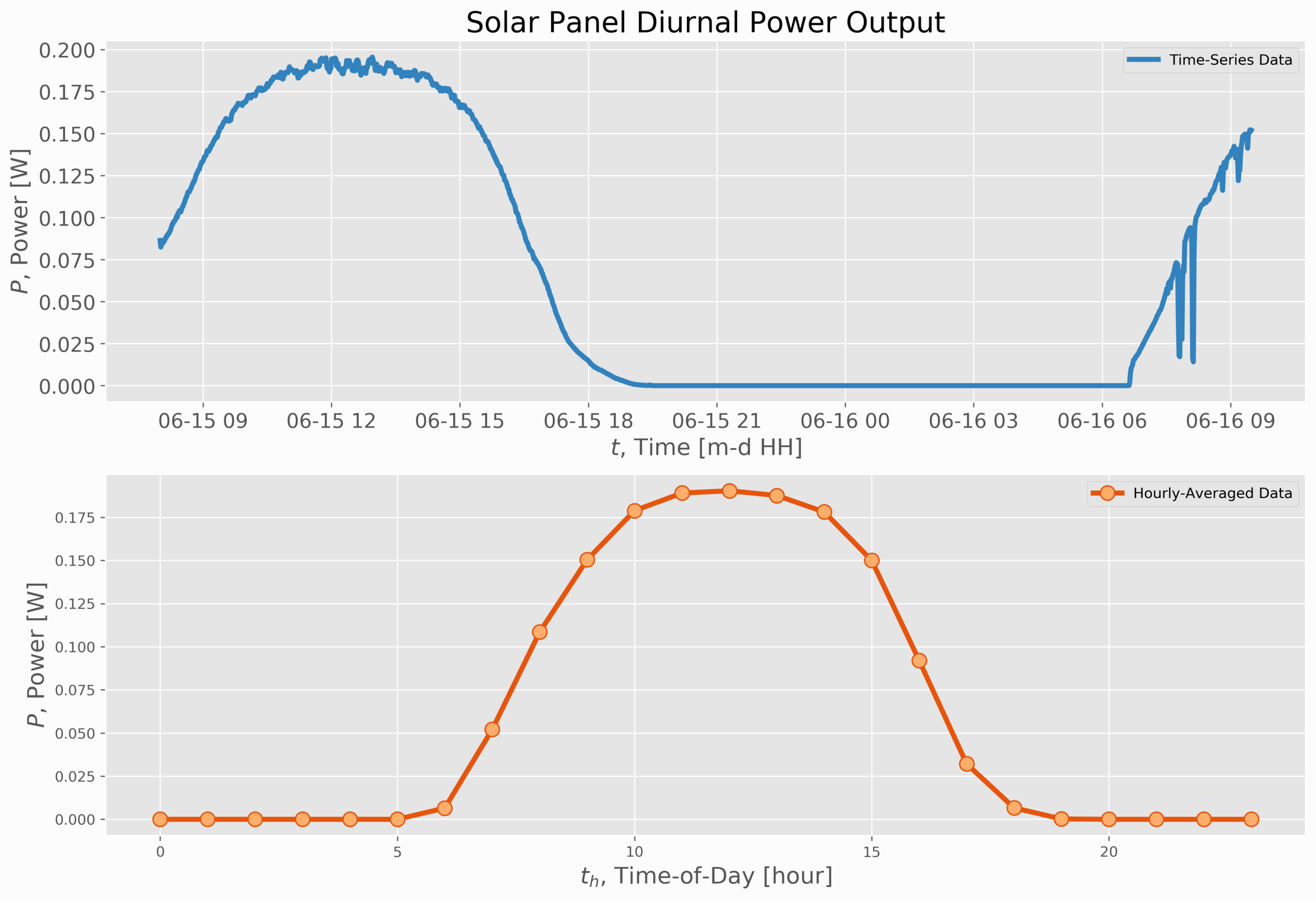
The top plot shows the raw time-series plot of the power output from the solar panel. There were a few drops in output on the morning of June 16th due to cloud cover, which is noted in the weather log for that morning:

Courtesy of Weather Underground: https://www.wunderground.com/history/daily/us/ca/san-francisco/KSFO/date/2021-6-16
The bottom portion of the plot shows the average diurnal output of the solar panel on an hourly basis. We can sum these values (since they are hourly) and call this value the daily solar output from the panel. Summing these values we get about 1.5W, which can be interpreted as 1.5W/day. Next, if we use the effective area of each solar cell, which in our case is 30mm x 10mm, multiplied by 4x (n = 4) because of the four cells in the panel, we can get the power density per day:
Finally, by assuming the panel material is of crystalline silicon, which is common for smaller and cheaper panels, we can predict an efficiency between 20%-25% (see solar efficiency tables for examples). With this efficiency in mind, we can make a very rough calculation of the incident solar insolation. Since solar insolation is fairly well documented, it will give us a decent idea of how the solar cell is performing. Dividing the power density above by an efficiency of 22% results in the following approximation of incident solar energy:
E0 ≈ 4.5 kWh/m2/day
As a check, we can find observations of solar insolation for San Francisco across the literature:
- Dey, Sumon, Madan Kumar Lakshmanan, and Bala Pesala. "Optimal solar tree design for increased flexibility in seasonal energy extraction." Renewable Energy 125 (2018). pp. 1038-1048.
- Mitchell, L., et al. "Impact of microclimates on solar resource: Case study of the solar resource in San Francisco." 2010 35th IEEE Photovoltaic Specialists Conference. IEEE, 2010.
- Karis, Robert. “San Francisco Solar Power Map.” (accessed June 16th, 2021).
The result calculated above tells us that our solar panel is operating as expected, under the assumption that its efficiency is somewhere around 20% and the solar insolation for the day of observation was somewhere around 4.6 kWh/
This tutorial focused on a real-world experiment involving a solar panel and Arduino datalogging system. The goal of this work was to explore how the electrical, physical, and solar variables affect the output measured by a solar panel. Using an Arduino board, SD datalogger, LiPo battery, and INA226 power meter - we were able to demonstrate the behavior and identify many of the characteristics of a solar panel. First, we varied the load at (near) peak solar insolation to identify the panel's nominal open-circuit voltage, short-circuit current, max power voltage and current, and max power output. These values helped us understand the optimal region of operation for the panel, while also opening the door for modeling and power prediction. We also conducted a daylong experiment that acquired data points every 60 seconds. Finally, we were able to identify the total daily power production and approximate the incident solar irradiation for the day. The experiment demonstrated the capabilities of Arduino, low-cost sensors, and the approachability of a real-world experiment with widely available hardware.

See more in Engineering and Arduino: