Water Metering with the WaWiCo USB Kit and Raspberry Pi

This is the second entry into the water metering tutorial series focused on the WaWiCo acoustic metering method. In the previous tutorial, the WaWiCo USB Water Metering Kit was introduced along with methods for listening to water flow through pipes without the need for invasive plumbing work. A Python GitHub repository was given that contains the signal processing codes used to analyze the incoming acoustic information emitted by the local piping system encompassed in the flexible band containing the MEMS microphone. For this project, we will be comparing the WaWiCo sensor with a conventional hall-effect mechanical flow meter. The WaWiCo sensor introduces a novel method for water metering, with non-invasive acoustic analysis. The benefit of the WaWiCo method is evident during the mechanical flow meter analysis, where we need to match pipe diameters and fittings and ensure that the flow terminates at a point. Otherwise, mechanical meters require cutting in piping — which is not an option for many users. Using a Raspberry Pi computer and a WaWiCo USB water meter kit, the frequency content of water flow for a given pipe is analyzed. Additionally, this frequency response will be used to correlate to the flow rate (in L/s) approximated by the mechanical flow meter. This brings us one step closer to being able to non-invasively measure water flow using the WaWiCo method.
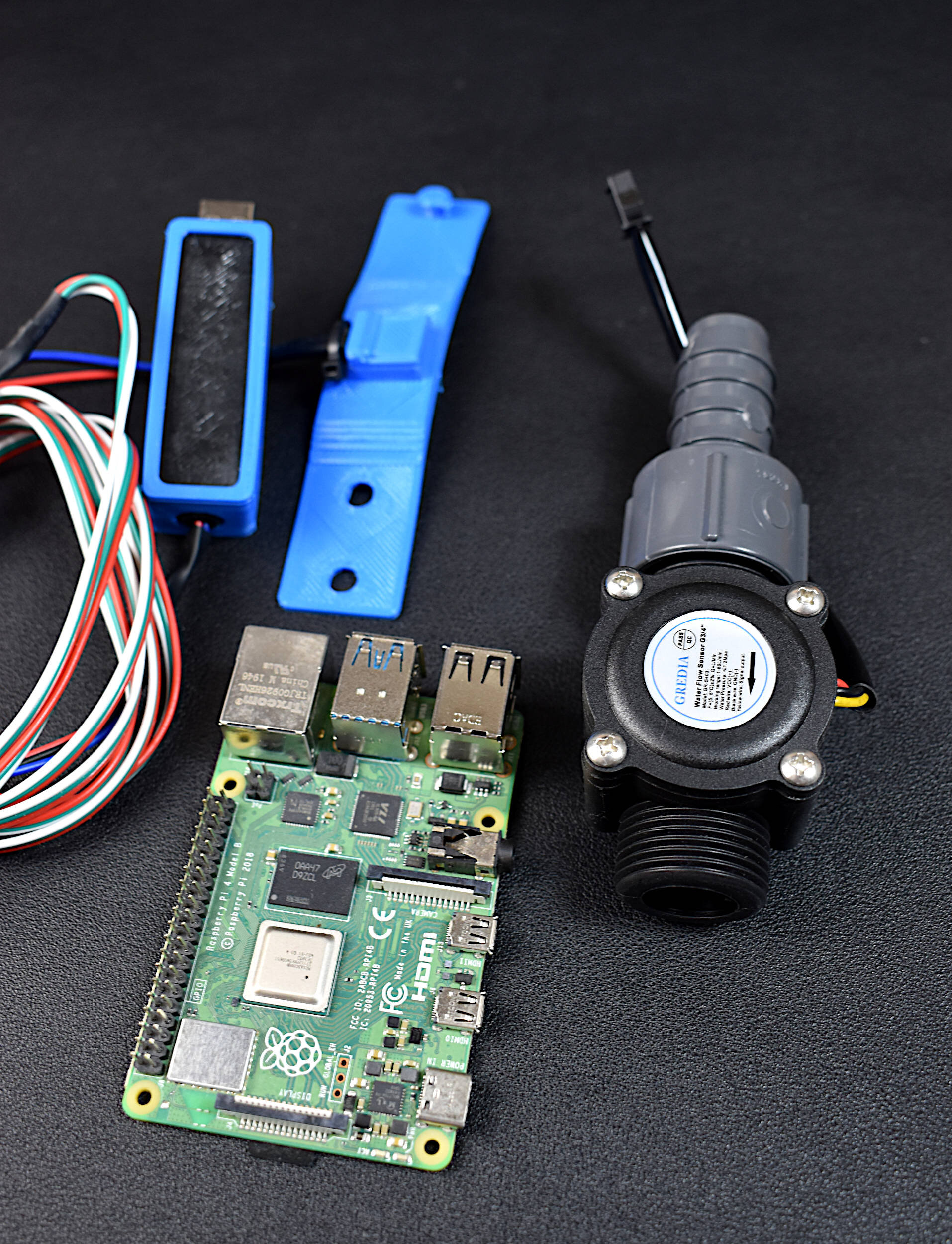
The main part used in this project is the WaWiCo USB Water Metering Kit, which can be found in our store in either pre-assmebled form or DIY kit form. The WaWiCo kit uses a MEMS microphone attached to the user’s piping system to listen for water flow via a computer’s USB port. A Raspberry Pi is used to read the USB signal in our case. Finally, a hall sensor water meter is used as a comparison against the acoustic WaWiCo device. The full parts list is given below to follow along in our analysis:
WaWiCo USB Water Metering Kit - $35 (Pre-Assembled), $20 (DIY Kit)
3/4" Hall Effect Flowmeter - $11.99 [Amazon]
3/4” Fitting, Barbed to NPT Female - $6.38 [Amazon]
3/4” ID Clear Vinyl Tubing - $24.99 (25ft) [Amazon]
Raspberry Pi 4 Computer - $52.99 (2GB), $61.88 (4GB), $88.50 (8GB) [Amazon], $55.00 [2GB from Our Store]

Water Wise Controls (WaWiCo) is a California-based company focused on water metering solutions using the acoustic profile of piping systems. Using this USB water metering kit, users can listen to their pipes and determine, based on advanced acoustic signal processing algorithms, whether water is flowing through a complex piping system. The USB metering kit includes a USB adapter for any PC and a flexible MEMS microphone band that can be attached to pipes ranging from 1”-2” in diameter.
Included in the USB Water Metering Kit:
1x MEMS Microphone
1x 6-ft 20AWG Connector Wire
1x USB Sound Card
3x 3D Printed Parts: USB Housing Case, Flexible USB Housing, Flexible MEMS Pipe Band
5V to 3.3V Voltage Regulator
Heat Shrink Tubing
2x JST Connector (1x Male, 1x Female)
Zip Tie for Flexband Securing
Features of the USB Water Metering Kit:
USB Sample Rate: 44.1kHz or 48kHz
16-bit Data Acquisition Precision
MEMS Microphone Frequency Response: 100Hz - 15kHz
Flexible Band for 1”-2” Diameter Piping
Compatible with Mac, Windows, and Linux-based Systems (Including Raspberry Pi)
For the DIY kit, the MEMS microphone needs to be powered from the USB sound card using the following pinout convention:

USB Type A Pinout for Powering the Regulator
The wiring, with the inclusion of the 3.3V regulator, is given below between the MEMS microphone and USB sound card:

Wiring Diagram for the DIY WaWiCo Water Metering Kit
In the pre-assembled kit, the wiring is done for the user.
For a detailed introduction, head to the first tutorial that covers many of the software installs required for the WaWiCo kit
An abridged version required for the software installation can be found at the WaWiCo USB Water Metering GitHub Page:

The flow meter being used as a comparison with the WaWiCo water metering kit must first be calibrated to ensure that the comparison between the two is valid. The way we calibrate the flow meter is by first looking at the relationship between the output signal and the actual flow rate measured by the actual fluid accumulation over time. For our flow meter, the relationship between flow rate and electronic output is given as follows:

Since we’re interested in shorter time periods (other than L/min), we can convert the approximation of flow rate Q in L/s:

If your calibration coefficient is not available, then the coefficient above may need to be calibrated. The way this can be done is through integration of the flow rate over time to a given measured volume. In our case, we are using a 3L container to measure water flowing through the mechanical flow meter. A photo of the flow meter and 3L container is shown below, for reference:

Mechanical Flow Meter Calibration with 3L Graduated Container
The code used to calibrate the flow meter is given below, which can also be found on the GitHub page:
##############################################
# Measuring water flow with mechanical flow
# meter for comparison against WaWiCo Acoustic
# flow detection
#
# -- by WaWiCo 2021
#
##############################################
#
import time,sys,signal
import RPi.GPIO as gpio
#
#####################################
# Functions for handling interrupt
#####################################
#
def signal_handler(sig,frame):
    gpio.cleanup()
    sys.exit(0)

def sensor_callback(chan):
    global counter
    counter+=1

if __name__== '__main__':
    #####################################
    # Experiment Parameter Setup
    #####################################
    #
    t_elapsed = 0.1 # time [s] between each flow rate calculation

    counter = 0 # for counting and calculating frequency

    Q_prev = 0.0 # previous flow calculation (for total flow calc.) [L/s]

    conv_factor = 1.0/(5.5*60) # conversion factor to [L/s] from freq [1/s or Hz]
    vol_approx = 0.0 # initial approximation of volume [L]
    vol_prev   = 0.0 # for minimizing the prints to console

    #####################################
    # GPIO setup for interrupt
    #####################################
    #
    sensor_gpio = 17 # sensor GPIO pin
    gpio.setmode(gpio.BCM) # set for GPIO pin configuration
    gpio.setup(sensor_gpio,gpio.IN,pull_up_down=gpio.PUD_UP) # set interrupt
    #
    #####################################
    # Interrupt setup
    #####################################
    #
    gpio.add_event_detect(sensor_gpio,gpio.FALLING,callback=sensor_callback,
                          bouncetime=1) # setup interrupt for event detection
    signal.signal(signal.SIGINT,signal_handler) # asynchronous interrupt handler
    #
    #####################################
    # Loop for approximating flow rate [L/s]
    # and total fluid accumulated [L]
    #####################################
    #
    t0 = time.time() # for updating time between calculations
    while True:
        if (time.time()-t0)<t_elapsed:
            pass
        else:
            Q = (conv_factor*(counter/t_elapsed)) # conversion to [Hz] then to [L/s]
            vol_approx+=(t_elapsed*((Q+Q_prev)/2.0)) # integrate over time for [L]
            counter = 0 # reset counter
            t0 = time.time() # get new time
            Q_prev = float(Q) # set previous rate
            if vol_approx!=vol_prev:
                print("Volume Approximation: {0:2.2f} L".format(vol_approx))
            vol_prev = float(vol_approx)
Below is a short GIF of the flow meter and calibration code running on a Raspberry Pi (ssh from laptop):

NOTE: If the mechanical flow meter registers output when there is no flow — a 0.1μF capacitor can be added between the signal and ground to remedy this noise
The variable ‘conv_factor = 1.0/(5.5*60)’ contains the sensor calibration coefficient, which in our case is 5.5. If the user is unaware or skeptical of their sensor calibration coefficient, this number should be altered based on a series of measurements at different volumes measured by the graduated container. For our sensor, the coefficient of 5.5 was correct and thus, we were able to verify it with several volumetric measurements using the script above. Therefore, going forward, we know that the code above with the calibration coefficient is accurate and can be used for flow measurement comparisons with the WaWiCo water metering kit.
Now that we have a mechanical flow meter for comparison working on the Raspberry Pi, we can start to look at the similarities and correlations between the mechanical flow meter and WaWico acoustic flow meter. This will allow us to establish correlations between the behavior we see from the mechanical meter and the acoustic meter positioned along the piping system or faucet (as we have it).

The code to correlate the two is also given below (and on the GitHub page), where the GPIO 23 on the Raspberry Pi is used to read the mechanical flow meter:
##############################################
# Measuring water flow with mechanical flow
# meter for comparison against WaWiCo Acoustic
# flow detection
#
# -- by WaWiCo 2021
#
##############################################
#
import time,sys,datetime
import signal as rpi_sig
import RPi.GPIO as gpio
import pyaudio
import matplotlib
matplotlib.use('TkAgg')
import matplotlib.pyplot as plt
import numpy as np
from scipy import signal
#
#####################################
# Functions for handling mechanical
# meter interrupts
#####################################
#
def signal_handler(sig,frame):
    gpio.cleanup()
    sys.exit(0)

def sensor_callback(chan):
    global counter
    counter+=1

##############################################
# function for FFT
##############################################
#
def fft_calc(data_vec):
    data_vec = butter_filt(data_vec)
    data_vec = data_vec*np.hanning(len(data_vec)) # hanning window
    N_fft = len(data_vec) # length of fft
    freq_vec = (float(samp_rate)*np.arange(0,int(N_fft/2)))/N_fft # fft frequency vector
    fft_data_raw = np.abs(np.fft.fft(data_vec)) # calculate FFT
    fft_data = fft_data_raw[0:int(N_fft/2)]/float(N_fft) # FFT amplitude scaling
    fft_data[1:] = 2.0*fft_data[1:] # single-sided FFT amplitude doubling
    return freq_vec,fft_data
##############################################
# Filtering Signal for Valid Bandpass
##############################################
#
def bandpass_coeffs():
    low_pt = frequency_bounds[0]/(0.5*samp_rate) # low freq cutoff relative to nyquist rate
    high_pt = frequency_bounds[1]/(0.5*samp_rate) # high freq cutoff relative to nyquist rate
    b,a = signal.butter(filt_order,[low_pt,high_pt],btype='band') # bandpass filter coeffs
    return b,a # return filter coefficients for bandpass

def butter_filt(data):
    b,a = bandpass_coeffs() # get filter coefficients
    data_filt = signal.lfilter(b,a,data) # data filter
    return data_filt
#
##############################################
# function for setting up pyserial
##############################################
#
def soundcard_finder(dev_indx=None,dev_name=None,dev_chans=1,dev_samprate=44100):
    ###############################
    # ---- look for USB sound card
    audio = pyaudio.PyAudio() # create pyaudio instantiation
    for dev_ii in range(audio.get_device_count()): # loop through devices
        dev = audio.get_device_info_by_index(dev_ii)
        if len(dev['name'].split('USB'))>1: # look for USB device
            dev_indx = dev['index'] # device index
            dev_name = dev['name'] # device name
            dev_chans = dev['maxInputChannels'] # input channels
            dev_samprate = dev['defaultSampleRate'] # sample rate
            print('PyAudio Device Info - Index: {0}, '.format(dev_indx)+\
                  'Name: {0}, Channels: {1:2.0f}, '.format(dev_name,dev_chans)+\
                      'Sample Rate {0:2.0f}'.format(samp_rate))
    if dev_name==None:
        print("No WaWico USB Device Found")
        return None,None,None
    return audio,dev_indx,dev_chans # return pyaudio, USB dev index, channels
#
def pyserial_start():
    ##############################
    ### create pyaudio stream  ###
    # -- streaming can be broken down as follows:
    # -- -- format             = bit depth of audio recording (16-bit is standard)
    # -- -- rate               = Sample Rate (44.1kHz, 48kHz, 96kHz)
    # -- -- channels           = channels to read (1-2, typically)
    # -- -- input_device_index = index of sound device
    # -- -- input              = True (let pyaudio know you want input)
    # -- -- frmaes_per_buffer  = chunk to grab and keep in buffer before reading
    ##############################
    stream = audio.open(format = pyaudio_format,rate = samp_rate,channels = chans, \
                        input_device_index = dev_indx,input = True, \
                        frames_per_buffer=CHUNK)
    stream.stop_stream() # stop stream to prevent overload
    return stream

def pyserial_end():
    stream.close() # close the stream
    audio.terminate() # close the pyaudio connection
#
##############################################
# functions for plotting data
##############################################
#
def spec_plotter():
    ##########################################
    # ---- spectrogram plot
    fig,ax = plt.subplots(figsize=(12,8)) # create figure
    ax.set_yscale('log') # log-scale for better visualization
    ax.set_ylim(frequency_bounds) # set frequency limits
    ax.set_xlabel('Time [s]',fontsize=16)# frequency label
    ax.set_ylabel('Frequency [Hz]',fontsize=16) # amplitude label

    fig.canvas.draw() # draw
    ax_bgnd = fig.canvas.copy_from_bbox(ax.bbox) # background for speedup
    spec1 = ax.pcolormesh(t_spectrogram,freq_array,fft_array,shading='auto') # plot
    fig.show() # show the figure
    return fig,ax,ax_bgnd,spec1

def plot_updater():
    ##########################################
    # ---- update spectrogram with new point
    fig.canvas.restore_region(ax_bgnd) # restore background
##    spec1.set_array(np.array(fft_array)[:-1,:-1].ravel()) # for shading='flat'
    spec1.set_array(np.array(fft_array).ravel()) # for shading='gouraud'
    ax.draw_artist(spec1) # re-draw spectrogram
    fig.canvas.blit(ax.bbox) # blit
    fig.canvas.flush_events() # for plotting
    return spec1
#
##############################################
# function for grabbing data from buffer
##############################################
#
def data_grabber():
    stream.start_stream() # start data stream
    t_0 = datetime.datetime.now() # get datetime of recording start
    data,data_frames = [],[] # variables
    for frame in range(0,update_samples):
        # grab data frames from buffer
        stream_data = stream.read(CHUNK,exception_on_overflow=False)
        data_frames.append(stream_data) # append data
        data.append(np.frombuffer(stream_data,dtype=buffer_format)/((2**15)-1))
    stream.stop_stream()
    return data,data_frames,t_0
#
##############################################
# function for analyzing data
##############################################
#
def data_analyzer():
    data_array = []
    t_ii = 0.0
    for frame in data_chunks:
        freq_ii,fft_ii = fft_calc(frame) # calculate fft for chunk
        fft_ii/=np.sqrt(np.mean(np.power(frame,2.0)))
        freq_array.append(freq_ii) # append chunk freq data to larger array
        fft_array.append(fft_ii) # append chunk fft data to larger array
        t_vec_ii = np.arange(0,len(frame))/float(samp_rate) # time vector
        t_ii+=t_vec_ii[-1]
        t_spectrogram.append(t_spectrogram[-1]) # time step for time v freq. plot
        data_array.extend(frame) # full data array
    t_vec = np.arange(0,len(data_array))/samp_rate # time vector for time series
    freq_vec,fft_vec = fft_calc(data_array) # fft of entire time series
    return t_vec,data_array,freq_vec,fft_vec,freq_array,fft_array,t_spectrogram

def corr_plot():
    #
    ###############################
    # Correlation Analysis between
    # Q and FFT data
    ###############################
    #
    x_vec = np.array(Q_corr_vec)
    y_vec = np.array(fft_corr_vec)
    y_vec_freq = np.array(freq_vec)

    xy_corr = []
    for ii in range(len(y_vec_freq)):
        xy_corr.append(np.sum((x_vec[:,ii]-np.mean(x_vec[:,ii]))*\
                              (y_vec[:,ii]-np.mean(y_vec[:,ii])))/\
                       (np.sqrt(np.sum(np.power(x_vec[:,ii]-np.mean(x_vec[:,ii]),2.0)))*\
                        np.sqrt(np.sum(np.power(y_vec[:,ii]-np.mean(y_vec[:,ii]),2.0)))))

    plt.style.use('ggplot')
    fig,ax = plt.subplots(figsize=(14,8))
    ax.scatter(y_vec_freq,xy_corr)
    ax.set_xscale('log')
    ax.set_xlim([1.0,samp_rate/2])
    ax.set_xlabel('Frequency [Hz]',fontsize=16)
    ax.set_ylabel(r'$\rho$',fontsize=16)
    return fig
#
##############################################
# Main Data Acquisition Procedure
##############################################
#
if __name__=="__main__":
    #####################################
    # Mechanical Flow Meter Setup
    #####################################
    #
    counter = 0 # for counting and calculating frequency

    Q_prev = 0.0 # previous flow calculation (for total flow calc.) [L/s]

    conv_factor = 1.0/(5.5*60) # conversion factor to [L/s] from freq [1/s or Hz]
    vol_approx = 0.0 # initial approximation of volume [L]
    vol_prev   = 0.0 # for minimizing the prints to console

    #####################################
    # GPIO setup for mechanical interrupt
    #####################################
    #
    sensor_gpio = 23 # sensor GPIO pin
    gpio.setmode(gpio.BCM) # set for GPIO pin configuration
    gpio.setup(sensor_gpio,gpio.IN,pull_up_down=gpio.PUD_UP) # set interrupt
    #
    #####################################
    # Interrupt setup
    #####################################
    #
    gpio.add_event_detect(sensor_gpio,gpio.FALLING,callback=sensor_callback,
                          bouncetime=1) # setup interrupt for event detection
    rpi_sig.signal(rpi_sig.SIGINT,signal_handler) # asynchronous interrupt handler
    #
    ################################
    # WaWiCo acquisition parameters
    ################################
    #
    CHUNK          = 2**12  # frames to keep in buffer between reads
    samp_rate      = 44100 # sample rate [Hz]
    pyaudio_format = pyaudio.paInt16 # 16-bit device
    buffer_format  = np.int16 # 16-bit for buffer
    #
    #############################
    # Find and Start Soundcard
    #############################
    #
    audio,dev_indx,chans = soundcard_finder() # start pyaudio,get indx,channels
    if audio == None:
        sys.exit() # exit if no WaWiCo sound card is found
    #
    #############################
    # stream info and data saver
    #############################
    #
    stream = pyserial_start() # start the pyaudio stream
    time_window = 10 # seconds within spectrogram window
    window_samples =  int((samp_rate*time_window)/CHUNK) # chunks to record
    update_window = 0.1
    update_samples = int((samp_rate*update_window)/CHUNK)

    plot_bool = 0 # boolean for first plot
    #
    ##############################
    # Pre-allocations for plot
    ##############################
    #
    freq_array = (float(samp_rate)*np.arange(0,int(CHUNK/2)))/CHUNK
    t_spectrogram = np.arange(window_samples)*CHUNK/samp_rate
    t_spectrogram = [np.repeat(ii,len(freq_array)) for ii in t_spectrogram]
    freq_array = [freq_array for ii in range(0,np.shape(t_spectrogram[0])[0])]
    fft_array = list(np.zeros(np.shape(t_spectrogram)))
    #
    ##############################
    # Frequency Window Filtering
    ##############################
    #
    frequency_bounds = [500.0,10000.0] # low/high frequency cutoffs
    filt_order = 5
    #
    #####################################
    #
    ##############################
    # Main Loop
    ##############################
    #
    #####################################
    #
    fft_corr_vec,Q_corr_vec = [],[]
    print('Recording Data...')
    print('Press CTRL+C to Finish Recording and Plot The Resulting Correlation')
    while True:
        try:
            counter = 0 # reset counter
            t0 = time.time()
            # get audio data
            data_chunks,data_frames,t_0 = data_grabber() # grab the audio data

            # mechanical flow section
            t_elapsed = time.time()-t0
            Q = (conv_factor*(counter/t_elapsed)) # conversion to [Hz] then to [L/s]
            vol_approx+=(t_elapsed*((Q+Q_prev)/2.0)) # integrate over time for [L]

            Q_prev = float(Q) # set previous rate
##            print("Flow Rate: {0:2.3f}[L/s], Volume : {1:2.3f} L".format(Q,vol_approx))
            vol_prev = float(vol_approx)

            # audio analysis section
            t_vec,data,freq_vec,fft_data,\
                    freq_array,fft_array,t_spectrogram = data_analyzer() # analyze recording

            fft_corr_vec.append(fft_data)
            Q_corr_vec.append(np.repeat(Q,np.shape(freq_vec)))
            # uncomment below for visualizing the frequency spectrum over time
    ##        if np.shape(t_spectrogram)[0]>window_samples:
    ##            freq_array = freq_array[-window_samples:] # remove first point
    ##            fft_array = fft_array[-window_samples:] # remove first point
    ##            t_spectrogram = t_spectrogram[-window_samples:] # remove first point
    ##            if plot_bool:
    ##                spec1 = plot_updater() # update spectrogram
    ##            else:
    ##                fig,ax,ax_bgnd,spec1 = spec_plotter() # first plot allocating params
    ##                plot_bool = 1 # lets the loop know the first plot started

        except:
            print('Plotting Correlation...')
            pyserial_end() # close the stream/pyaudio connection
            fig = corr_plot()
            fig.savefig('./images/wawico_mechanical_correlation.png',dpi=300,bbox_inches='tight',
                        facecolor='#FCFCFC')
            fig.savefig('./images/wawico_mechanical_correlation_white.png',dpi=300,bbox_inches='tight',
                        facecolor='#FFFFFF')
            plt.show()
            break
An example plot from the correlation analysis is given below:

In our example plot above, our correlation between our faucet mechanical flow rate and our WaWiCo acoustic signal shows fairly high correlation, ρ = 0.85, for the region 5kHz-8kHz, and perhaps 10kHz+, with a region of anti-correlation in the 9kHz region. This is important for monitoring flow in the future, as we can monitor this region and determine if water is flowing or not.
Note #1: the correlation coefficient ranges from -1 to +1, where +1 indicates the two signals are correlated and -1 indicates the two signals are negatively correlated. Ideally, we want the highest correlation either in the positive or negative direction, as the higher value indicates a better correlation between the two signals (even if negatively, i.e. in opposite sign).
Note #2: Another important note is that the longer the script runs, the more information the analysis will have for analyzing the piping system and correlation between mechanical flow meter and acoustic response. That being said - there also must be a diverse set of data inputted to the system, meaning - no flow periods, water flow periods, background noise and disturbances indicative of the normal environment need to be part of the testing. This will create a better correlation between the response and actual flow, while minimizing interference and false-trips during noisy non-flow periods.
In this section, we implement a Goertzel algorithm for finding the power contained within a frequency range found from above. Then, this power is used to compare with the mechanical flow meter in order to determine the viability of water metering using the amplitude of the response from the Goertzel calculation.
The code used to acquire both the frequency band from the Goertzel algorithm and the flow rate from the mechanical meter is given below (and on the project GitHub page):
##############################################
# Measuring water flow with mechanical flow
# meter for comparison against WaWiCo Acoustic
# flow detection
#
# -- by WaWiCo 2021
#
##############################################
#
import time,sys,datetime
import signal as rpi_sig
import RPi.GPIO as gpio
import pyaudio
import matplotlib
matplotlib.use('TkAgg')
import matplotlib.pyplot as plt
import numpy as np
from scipy import signal
#
#####################################
# Functions for handling mechanical
# meter interrupts
#####################################
#
def signal_handler(sig,frame):
    gpio.cleanup()
    sys.exit(0)

def sensor_callback(chan):
    global counter
    counter+=1

##############################################
# function for FFT
##############################################
#
def fft_calc(data_vec):
    data_vec = butter_filt(data_vec)
    data_vec = data_vec*np.hanning(len(data_vec)) # hanning window
    N_fft = len(data_vec) # length of fft
    freq_vec = (float(samp_rate)*np.arange(0,int(N_fft/2)))/N_fft # fft frequency vector
    fft_data_raw = np.abs(np.fft.fft(data_vec)) # calculate FFT
    fft_data = fft_data_raw[0:int(N_fft/2)]/float(N_fft) # FFT amplitude scaling
    fft_data[1:] = 2.0*fft_data[1:] # single-sided FFT amplitude doubling
    return freq_vec,fft_data
##############################################
# Filtering Signal for Valid Bandpass
##############################################
#
def bandpass_coeffs():
    low_pt = frequency_bounds[0]/(0.5*samp_rate) # low freq cutoff relative to nyquist rate
    high_pt = frequency_bounds[1]/(0.5*samp_rate) # high freq cutoff relative to nyquist rate
    b,a = signal.butter(filt_order,[low_pt,high_pt],btype='band') # bandpass filter coeffs
    return b,a # return filter coefficients for bandpass

def butter_filt(data):
    b,a = bandpass_coeffs() # get filter coefficients
    data_filt = signal.lfilter(b,a,data) # data filter
    return data_filt
#
##############################################
# function for setting up pyserial
##############################################
#
def soundcard_finder(dev_indx=None,dev_name=None,dev_chans=1,dev_samprate=44100):
    ###############################
    # ---- look for USB sound card
    audio = pyaudio.PyAudio() # create pyaudio instantiation
    for dev_ii in range(audio.get_device_count()): # loop through devices
        dev = audio.get_device_info_by_index(dev_ii)
        if len(dev['name'].split('USB'))>1: # look for USB device
            dev_indx = dev['index'] # device index
            dev_name = dev['name'] # device name
            dev_chans = dev['maxInputChannels'] # input channels
            dev_samprate = dev['defaultSampleRate'] # sample rate
            print('PyAudio Device Info - Index: {0}, '.format(dev_indx)+\
                  'Name: {0}, Channels: {1:2.0f}, '.format(dev_name,dev_chans)+\
                      'Sample Rate {0:2.0f}'.format(samp_rate))
    if dev_name==None:
        print("No WaWico USB Device Found")
        return None,None,None
    return audio,dev_indx,dev_chans # return pyaudio, USB dev index, channels
#
def pyserial_start():
    ##############################
    ### create pyaudio stream  ###
    # -- streaming can be broken down as follows:
    # -- -- format             = bit depth of audio recording (16-bit is standard)
    # -- -- rate               = Sample Rate (44.1kHz, 48kHz, 96kHz)
    # -- -- channels           = channels to read (1-2, typically)
    # -- -- input_device_index = index of sound device
    # -- -- input              = True (let pyaudio know you want input)
    # -- -- frmaes_per_buffer  = chunk to grab and keep in buffer before reading
    ##############################
    stream = audio.open(format = pyaudio_format,rate = samp_rate,channels = chans, \
                        input_device_index = dev_indx,input = True, \
                        frames_per_buffer=CHUNK)
    stream.stop_stream() # stop stream to prevent overload
    return stream

def pyserial_end():
    stream.close() # close the stream
    audio.terminate() # close the pyaudio connection
#
##############################################
# functions for plotting data
##############################################
#
def spec_plotter():
    ##########################################
    # ---- spectrogram plot
    fig,ax = plt.subplots(figsize=(12,8)) # create figure
    ax.set_yscale('log') # log-scale for better visualization
    ax.set_ylim(frequency_bounds) # set frequency limits
    ax.set_xlabel('Time [s]',fontsize=16)# frequency label
    ax.set_ylabel('Frequency [Hz]',fontsize=16) # amplitude label

    fig.canvas.draw() # draw
    ax_bgnd = fig.canvas.copy_from_bbox(ax.bbox) # background for speedup
    spec1 = ax.pcolormesh(t_spectrogram,freq_array,fft_array,shading='auto') # plot
    fig.show() # show the figure
    return fig,ax,ax_bgnd,spec1

def plot_updater():
    ##########################################
    # ---- update spectrogram with new point
    fig.canvas.restore_region(ax_bgnd) # restore background
##    spec1.set_array(np.array(fft_array)[:-1,:-1].ravel()) # for shading='flat'
    spec1.set_array(np.array(fft_array).ravel()) # for shading='gouraud'
    ax.draw_artist(spec1) # re-draw spectrogram
    fig.canvas.blit(ax.bbox) # blit
    fig.canvas.flush_events() # for plotting
    return spec1
#
##############################################
# function for grabbing data from buffer
##############################################
#
def data_grabber():
    stream.start_stream() # start data stream
    t_0 = datetime.datetime.now() # get datetime of recording start
    data,data_frames = [],[] # variables
    for frame in range(0,update_samples):
        # grab data frames from buffer
        stream_data = stream.read(CHUNK,exception_on_overflow=False)
        data_frames.append(stream_data) # append data
        data.append(np.frombuffer(stream_data,dtype=buffer_format)/((2**15)-1))
    stream.stop_stream()
    return data,data_frames,t_0
#
##############################################
# function for analyzing data
##############################################
#
def data_analyzer():
    data_array = []
    t_ii = 0.0
    for frame in data_chunks:
        freq_ii,fft_ii = fft_calc(frame) # calculate fft for chunk
        fft_ii/=np.sqrt(np.mean(np.power(frame,2.0)))
        freq_array.append(freq_ii) # append chunk freq data to larger array
        fft_array.append(fft_ii) # append chunk fft data to larger array
        t_vec_ii = np.arange(0,len(frame))/float(samp_rate) # time vector
        t_ii+=t_vec_ii[-1]
        t_spectrogram.append(t_spectrogram[-1]) # time step for time v freq. plot
        data_array.extend(frame) # full data array
    t_vec = np.arange(0,len(data_array))/samp_rate # time vector for time series
    freq_vec,fft_vec = fft_calc(data_array) # fft of entire time series
    return t_vec,data_array,freq_vec,fft_vec,freq_array,fft_array,t_spectrogram

def corr_plot():
    #
    ###############################
    # Correlation Analysis between
    # Q and FFT data
    ###############################
    #
    x_vec = np.array(Q_corr_vec)
    y_vec = np.array(fft_corr_vec)
    y_vec_freq = np.array(freq_vec)

    xy_corr = []
    for ii in range(len(y_vec_freq)):
        xy_corr.append(np.sum((x_vec[:,ii]-np.mean(x_vec[:,ii]))*\
                              (y_vec[:,ii]-np.mean(y_vec[:,ii])))/\
                       (np.sqrt(np.sum(np.power(x_vec[:,ii]-np.mean(x_vec[:,ii]),2.0)))*\
                        np.sqrt(np.sum(np.power(y_vec[:,ii]-np.mean(y_vec[:,ii]),2.0)))))

    plt.style.use('ggplot')
    fig,ax = plt.subplots(figsize=(14,8))
    ax.scatter(y_vec_freq,xy_corr)
    ax.set_xscale('log')
    ax.set_xlim([1.0,samp_rate/2])
    ax.set_xlabel('Frequency [Hz]',fontsize=16)
    ax.set_ylabel(r'$\rho$',fontsize=16)
    return fig

def Q_vs_goertzel_plot(freq_band_ii):
    #
    ###############################
    # Plot Comparison between
    # Q and Goertzel Response
    ###############################
    #
    x_vec = np.array(Q_vec)
    y_vec = np.array(goertzel_vec)

    plt.style.use('ggplot')
    fig,ax = plt.subplots(figsize=(14,8))
    ax.scatter(x_vec,y_vec)
    ax.set_xlabel('$Q$ [L/s]',fontsize=16)
    ax.set_ylabel('Summed Goertzel Amplitude ({0:2.1f}kHz - {1:2.1f}kHz)'.format(freq_band_ii[0]/1000.0,
                                                        freq_band_ii[1]/1000.0),fontsize=16)
    return fig

################################################################################
# Goertzel DFT/FFT  module    From
# https://stackoverflow.com/questions/13499852/scipy-fourier-transform-of-a-few-selected-frequencies
################################################################################
def goertzel(samples, sample_rate, *freqs):
    #usage: freqs, results = goertzel(some_samples, 44100, (400, 500), (1000, 1100))
    window_size = len(samples)
    f_step = sample_rate/float(window_size)
    f_step_normalized = 1.0 / window_size

    # Calculate all the DFT bins we have to compute to include frequencies
    # in `freqs`.
    bins = set()
    for f_range in freqs:
        f_start, f_end = f_range
        k_start = int(np.floor(f_start / f_step))
        k_end = int(np.ceil(f_end / f_step))

        if k_end > window_size - 1: raise ValueError('frequency out of range %s' % k_end)
        bins = bins.union(range(k_start, k_end))

    # For all the bins, calculate the DFT term
    n_range = range(0, window_size)
    freqs = []
    results = []
    for k in bins:

        # Bin frequency and coefficients for the computation
        f = k * f_step_normalized
        w_real = 2.0 * np.cos(2.0 * np.pi * f)
        w_imag = np.sin(2.0 * np.pi * f)

        # Doing the calculation on the whole sample
        d1, d2 = 0.0, 0.0
        for n in n_range:
            y  = samples[n] + w_real * d1 - d2
            d2, d1 = d1, y

        # Storing results `(real part, imag part, power)`
        results.append([0.5 * w_real * d1 - d2,
                        w_imag * d1,
                        d2**2 + d1**2 - w_real * d1 * d2])
        freqs.append(f * sample_rate)
    return freqs, results

#
##############################################
# Main Data Acquisition Procedure
##############################################
#
if __name__=="__main__":
    #####################################
    # Mechanical Flow Meter Setup
    #####################################
    #
    counter = 0 # for counting and calculating frequency

    Q_prev = 0.0 # previous flow calculation (for total flow calc.) [L/s]

    conv_factor = 1.0/(5.5*60) # conversion factor to [L/s] from freq [1/s or Hz]
    vol_approx = 0.0 # initial approximation of volume [L]
    vol_prev   = 0.0 # for minimizing the prints to console

    #####################################
    # GPIO setup for mechanical interrupt
    #####################################
    #
    sensor_gpio = 23 # sensor GPIO pin
    gpio.setmode(gpio.BCM) # set for GPIO pin configuration
    gpio.setup(sensor_gpio,gpio.IN,pull_up_down=gpio.PUD_UP) # set interrupt
    #
    #####################################
    # Interrupt setup
    #####################################
    #
    gpio.add_event_detect(sensor_gpio,gpio.FALLING,callback=sensor_callback,
                          bouncetime=1) # setup interrupt for event detection
    rpi_sig.signal(rpi_sig.SIGINT,signal_handler) # asynchronous interrupt handler
    #
    ################################
    # WaWiCo acquisition parameters
    ################################
    #
    CHUNK          = 2**12  # frames to keep in buffer between reads
    samp_rate      = 44100 # sample rate [Hz]
    pyaudio_format = pyaudio.paInt16 # 16-bit device
    buffer_format  = np.int16 # 16-bit for buffer
    #
    #############################
    # Find and Start Soundcard
    #############################
    #
    audio,dev_indx,chans = soundcard_finder() # start pyaudio,get indx,channels
    if audio == None:
        sys.exit() # exit if no WaWiCo sound card is found
    #
    #############################
    # stream info and data saver
    #############################
    #
    stream = pyserial_start() # start the pyaudio stream
    time_window = 10 # seconds within spectrogram window
    window_samples =  int((samp_rate*time_window)/CHUNK) # chunks to record
    update_window = 0.1
    update_samples = int((samp_rate*update_window)/CHUNK)

    plot_bool = 0 # boolean for first plot
    #
    ##############################
    # Pre-allocations for plot
    ##############################
    #
    freq_array = (float(samp_rate)*np.arange(0,int(CHUNK/2)))/CHUNK
    t_spectrogram = np.arange(window_samples)*CHUNK/samp_rate
    t_spectrogram = [np.repeat(ii,len(freq_array)) for ii in t_spectrogram]
    freq_array = [freq_array for ii in range(0,np.shape(t_spectrogram[0])[0])]
    fft_array = list(np.zeros(np.shape(t_spectrogram)))
    #
    ##############################
    # Frequency Window Filtering
    ##############################
    #
    frequency_bounds = [500.0,10000.0] # low/high frequency cutoffs
    filt_order = 5
    #
    #####################################
    #
    ##############################
    # Main Loop
    ##############################
    #
    #####################################
    #
    goertzel_vec,Q_vec = [],[]
    print('Recording Data...')
    print('Press CTRL+C to Finish Recording and Plot The Resulting Correlation')
    while True:
        try:
            counter = 0 # reset counter
            t0 = time.time()
            # get audio data
            data_chunks,data_frames,t_0 = data_grabber() # grab the audio data

            # mechanical flow section
            t_elapsed = time.time()-t0
            Q = (conv_factor*(counter/t_elapsed)) # conversion to [Hz] then to [L/s]
            vol_approx+=(t_elapsed*((Q+Q_prev)/2.0)) # integrate over time for [L]

            Q_prev = float(Q) # set previous rate
##            print("Flow Rate: {0:2.3f}[L/s], Volume : {1:2.3f} L".format(Q,vol_approx))
            vol_prev = float(vol_approx)

            # audio analysis section
            t_vec,data,freq_vec,fft_data,\
                    freq_array,fft_array,t_spectrogram = data_analyzer() # analyze recording

            freq_band = (7500.0,8500.0)
            freqs,goertzel_data = goertzel(data
                                       , samp_rate, freq_band)

            goertzel_vec.append(np.sum(np.array(goertzel_data)[:,2]))
            Q_vec.append(Q)

        except:
            print('Plotting Data...')
            pyserial_end() # close the stream/pyaudio connection
            fig = Q_vs_goertzel_plot(freq_band)
            plt.show()
            break
The Goertzel algorithm is often used to evaluate a selected frequency band of terms of the Fast Fourier Transform (FFT) [read more about the Goertzel algorithm and its applications in acoustics here]. Parameters of the Goertzel algorithm, such as the spacing between frequencies is controlled by the sample rate and the recording length of the audio signal. The specifics of the Goertzel algorithm are not covered here, but the function contains comments that explains some of the procedure.
Below is an example output of the analysis done to compare the Goertzel response over the 7.5kHz - 8.5kHz region and the mechanical flow meter:

The plot above allows us to make several statements about the relationship between flow rate and power in the frequency bands of interest:
When the flow rate is low, the acoustic device shows little amplitude change
Each flow rate has a range of Goertzel amplitudes that indicate flow
The algorithm is not susceptible to false positives (i.e. no flow = very low Goertzel amplitude)
It may be hard to distinguish between flow rates, but more needs to be done to verify this (perhaps different frequency bands can determine this?)
The flow meter is not very sensitive over the short term period used here ( ≈ 93ms), perhaps longer periods could give better resolution in Q
The faucet being used is somewhat turbulent, which may describe the difficulty of resolving flow at higher flow rates
The experiment above can also be run for different frequency ranges, which may contain more information
A possible explanation for the wide Goertzel response in the middle flow rates may be explained by lags between audio input and mechanical flow meter
In this tutorial, a mechanical flow meter was introduced as a comparison to the WaWiCo USB Water Metering Kit. The WaWiCo USB kit listens to your pipes via an acoustic signal, while the mechanical meter uses the actual flow of water to approximate flow rate. The goal of this tutorial was to bring the WaWiCo acoustic listening method closer to an actual water meter by developing routines that correlate the mechanical flow of water through a hall-effect turbine to the acoustic vibration or water flow measured by the WaWiCo flexible acoustic device attached to the piping system. The advantage of the WaWiCo method is that it requires no changes to the user’s piping system. No plumbing required, no invasive cutting, and no disruption to the user’s daily water use. Conversely, the mechanical flow meter must be placed inline with the flow. This is the great advantage to the WaWiCo method and the USB water metering device!

See more from WaWiCo:


