Accelerometer, Gyroscope, and Magnetometer Analysis with Raspberry Pi Part I: Basic Readings
“As an Amazon Associates Program member, clicking on links may result in Maker Portal receiving a small commission that helps support future projects.”
The MPU9250 is a powerful inertial measurement unit (IMU) consisting of three primary sensors: an accelerometer, a gyroscope, and a magnetometer. Each sensor measures a 3-axis signal in the cartesian reference x,y,z. Each of the 9-degrees of freedom is converted into a 16-bit digital signal, which can be read at different speeds depending on the sensor. The accelerometer is capable of measuring ±2, ±4, ±8, and ±16g at a sample rate of 1 kHz, the gyroscope can measure ±250°/s, ±500°/s, ±1000°/s, and ±2000°/s (dps or degrees per second) at a sample rate of 8 kHz, and the magnetometer can measure ±4800μT at 100 Hz.
A Raspberry Pi will be used to read the MPU9250 3-axis acceleration, 3-axis angular rotation speed, and 3-axis magnetic flux (MPU9250 product page can be found here). The output and limitations of the MPU9250 will be explored, which will help define the limitations of applications for each sensor. This is only the first entry into the MPU9250 IMU series, where in the breadth of the articles we will apply advanced techniques in Python to analyze each of the 9-axes of the IMU and develop real-world applications for the sensor, which may be useful to engineers interested in vibration analysis, navigation, vehicle control, and many other areas.
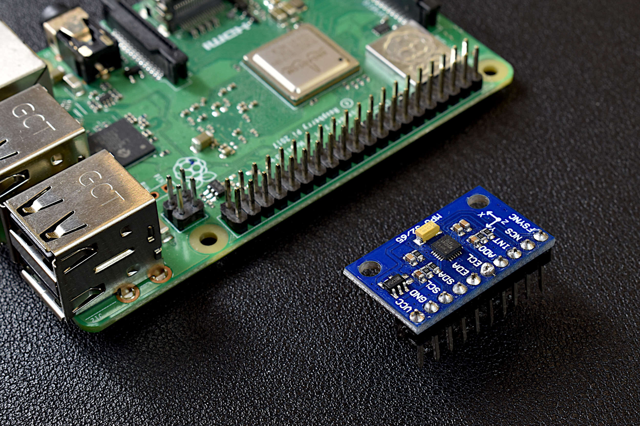
This tutorial uses two primary components: An MPU9250 9-DoF IMU and a Raspberry Pi computer. Any Rapsberry Pi will do as long as it has I2C communication and is capable of running Python 3.x. I have listed the parts and where I purchased them below, along with some other components that may make following along with the tutorial more seamless:
Raspberry Pi 4 Computer - $38.40 - $62.00 [1GB on Amazon, 2GB Amazon, 4GB Amazon], $55.00 [2GB from Our Store]
MPU9250 IMU - $13.00 [Our Store]
Mini Breadboard - $3.00 [Our Store]
Jumper Wires - $0.90 (6 pcs) [Our Store]
Raspberry Pi 4 Kit (HDMI cables, USB cables, etc.) - $97.99 [Amazon]

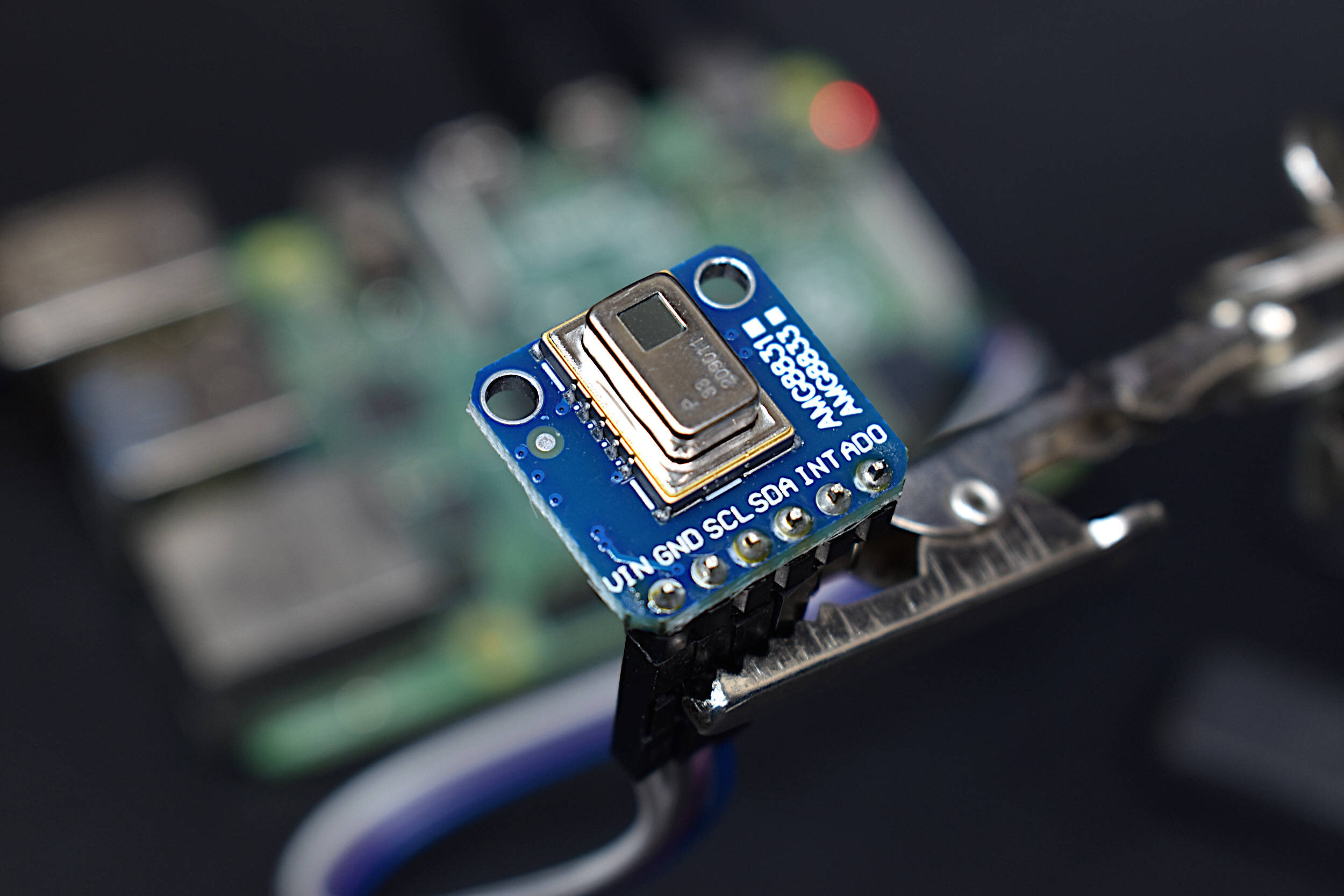
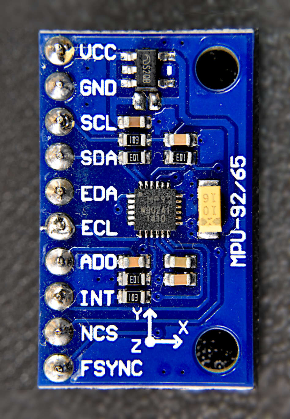
The wiring digram for the MPU9250 and Raspberry Pi is given below (and in the neighboring table). In actuality, I will be using the Rapsberry Pi 4 (despite the diagram stating it is a RPi 3), however the pinout and protocols are all the same. Take note of the second I2C (EDA/ECL) wiring - this is important because it wires both the MPU6050 (accelerometer/gyroscope) and AK8963 (magnetometer) to the RPi’s I2C port. This also means that we will be communicating with two I2C devices (more on this later).
| RPI Pin | MPU9250 Pin |
|---|---|
| 3.3V (1) | VCC |
| GND (6) | GND |
| SDA (3) | SDA |
| SCL (5) | SCL |
| ECL → SCL | |
| EDA → SDA |
The MPU9250 will communicate with the Raspberry Pi using the I2C protocol. In order to read and write data via I2C, we must first enable the I2C ports on the RPi. The way we do this is either using the command line or by navigating to the Preferences → Raspberry Pi Configuration. Adafruit has a great tutorial outlining this process, but an abridged version will be given below using screenshots of the RPi configuration window.

1. Preferences → Raspberry Pi Configuration
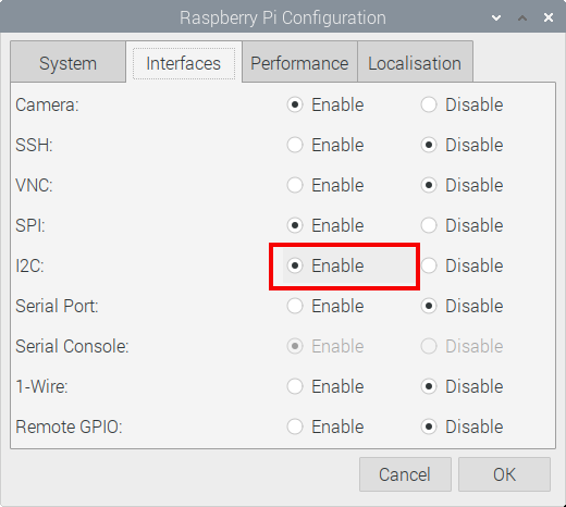
2. Interfaces → Enable I2C

3. Open Command Window and type “sudo i2cdetect -y 1”
Verify 0x68 (MPU6050) and 0x0C (AK8963) as I2C devices
Once both MPU9250 devices show up on the I2C detector in the RPi command window, we are ready to read the MPU6050 (0x68 device address) and AK8963 (0x0C device address). The reason why we need both addresses is that we have wired them to the same I2C port, so we now use their addresses to control them in a program. In this tutorial, Python will be used. The device addresses can be found in their respective datasheets or by testing them individually by wiring them one-by-one. We know that the MPU6050 (accel/gyro) is 0x68 from its datasheet, and we know the AK8963 (magnetometer) is 0x0C from its datasheet, so the wiring test is not necessary.
If you only see one device address, recheck the wiring; and if no devices are showing up also check the wiring and ensure there is power to the MPU9250 and also that the I2C has been enabled on the RPi! Going forward, it is assumed that the MPU9250 has been wired to the RPi and that the device addresses are identical to the ones given above. Of course, we can easily change the device addresses in the Python code, so if your device for some reason has different addresses, the user will need to change that in the codes that follow.
Lastly, we will need to increase the speed of the I2C baud rate in order to get the fastest response from the MPU9250, which we can do by entering the following into the command line:

1. sudo nano /boot/config.txt

2. Add Line in Next to I2C Setting
All we are doing here is setting the baud rate to 1 Mbps. This should give us a sample rate of about 400Hz - 500Hz (after conversion to real-world units). We can achieve a much higher sample rate for the gyroscope and a slightly higher sample rate for the accelerometer, but that will not be explored in this series.

In Python, the I2C port can be accessed using a particular library called ‘smbus.’ The smbus is intialized using the following simple routine:
import smbus
bus = smbus.SMBus(1)
Using the ‘bus’ specified in the code above, we will use the MPU9250 Register Map document to gives us information about how to communicate with the accelerometer, gyroscope, and magnetometer (MPU6050 and AK8963). The I2C bus methods used in Python are outside of the scope of this tutorial, so they will not be described in great detail; therefore, the code used to communicate back and forth to the MPU6050 and AK8963 are given below without much description. The full details and capabilities of each sensor are given in the datasheet to the MPU9250, where many questions regarding the registers and corresponding values can be explored, if desired.
# this is to be saved in the local folder under the name "mpu9250_i2c.py"
# it will be used as the I2C controller and function harbor for the project
# refer to datasheet and register map for full explanation

import smbus,time

def MPU6050_start():
    # alter sample rate (stability)
    samp_rate_div = 0 # sample rate = 8 kHz/(1+samp_rate_div)
    bus.write_byte_data(MPU6050_ADDR, SMPLRT_DIV, samp_rate_div)
    time.sleep(0.1)
    # reset all sensors
    bus.write_byte_data(MPU6050_ADDR,PWR_MGMT_1,0x00)
    time.sleep(0.1)
    # power management and crystal settings
    bus.write_byte_data(MPU6050_ADDR, PWR_MGMT_1, 0x01)
    time.sleep(0.1)
    #Write to Configuration register
    bus.write_byte_data(MPU6050_ADDR, CONFIG, 0)
    time.sleep(0.1)
    #Write to Gyro configuration register
    gyro_config_sel = [0b00000,0b010000,0b10000,0b11000] # byte registers
    gyro_config_vals = [250.0,500.0,1000.0,2000.0] # degrees/sec
    gyro_indx = 0
    bus.write_byte_data(MPU6050_ADDR, GYRO_CONFIG, int(gyro_config_sel[gyro_indx]))
    time.sleep(0.1)
    #Write to Accel configuration register
    accel_config_sel = [0b00000,0b01000,0b10000,0b11000] # byte registers
    accel_config_vals = [2.0,4.0,8.0,16.0] # g (g = 9.81 m/s^2)
    accel_indx = 0
    bus.write_byte_data(MPU6050_ADDR, ACCEL_CONFIG, int(accel_config_sel[accel_indx]))
    time.sleep(0.1)
    # interrupt register (related to overflow of data [FIFO])
    bus.write_byte_data(MPU6050_ADDR, INT_ENABLE, 1)
    time.sleep(0.1)
    return gyro_config_vals[gyro_indx],accel_config_vals[accel_indx]

def read_raw_bits(register):
    # read accel and gyro values
    high = bus.read_byte_data(MPU6050_ADDR, register)
    low = bus.read_byte_data(MPU6050_ADDR, register+1)

    # combine higha and low for unsigned bit value
    value = ((high << 8) | low)

    # convert to +- value
    if(value > 32768):
        value -= 65536
    return value

def mpu6050_conv():
    # raw acceleration bits
    acc_x = read_raw_bits(ACCEL_XOUT_H)
    acc_y = read_raw_bits(ACCEL_YOUT_H)
    acc_z = read_raw_bits(ACCEL_ZOUT_H)

    # raw temp bits
##    t_val = read_raw_bits(TEMP_OUT_H) # uncomment to read temp

    # raw gyroscope bits
    gyro_x = read_raw_bits(GYRO_XOUT_H)
    gyro_y = read_raw_bits(GYRO_YOUT_H)
    gyro_z = read_raw_bits(GYRO_ZOUT_H)

    #convert to acceleration in g and gyro dps
    a_x = (acc_x/(2.0**15.0))*accel_sens
    a_y = (acc_y/(2.0**15.0))*accel_sens
    a_z = (acc_z/(2.0**15.0))*accel_sens

    w_x = (gyro_x/(2.0**15.0))*gyro_sens
    w_y = (gyro_y/(2.0**15.0))*gyro_sens
    w_z = (gyro_z/(2.0**15.0))*gyro_sens

##    temp = ((t_val)/333.87)+21.0 # uncomment and add below in return
    return a_x,a_y,a_z,w_x,w_y,w_z

def AK8963_start():
    bus.write_byte_data(AK8963_ADDR,AK8963_CNTL,0x00)
    time.sleep(0.1)
    AK8963_bit_res = 0b0001 # 0b0001 = 16-bit
    AK8963_samp_rate = 0b0110 # 0b0010 = 8 Hz, 0b0110 = 100 Hz
    AK8963_mode = (AK8963_bit_res <<4)+AK8963_samp_rate # bit conversion
    bus.write_byte_data(AK8963_ADDR,AK8963_CNTL,AK8963_mode)
    time.sleep(0.1)

def AK8963_reader(register):
    # read magnetometer values
    low = bus.read_byte_data(AK8963_ADDR, register-1)
    high = bus.read_byte_data(AK8963_ADDR, register)
    # combine higha and low for unsigned bit value
    value = ((high << 8) | low)
    # convert to +- value
    if(value > 32768):
        value -= 65536
    return value

def AK8963_conv():
    # raw magnetometer bits

    loop_count = 0
    while 1:
        mag_x = AK8963_reader(HXH)
        mag_y = AK8963_reader(HYH)
        mag_z = AK8963_reader(HZH)

        # the next line is needed for AK8963
        if bin(bus.read_byte_data(AK8963_ADDR,AK8963_ST2))=='0b10000':
            break
        loop_count+=1

    #convert to acceleration in g and gyro dps
    m_x = (mag_x/(2.0**15.0))*mag_sens
    m_y = (mag_y/(2.0**15.0))*mag_sens
    m_z = (mag_z/(2.0**15.0))*mag_sens

    return m_x,m_y,m_z

# MPU6050 Registers
MPU6050_ADDR = 0x68
PWR_MGMT_1   = 0x6B
SMPLRT_DIV   = 0x19
CONFIG       = 0x1A
GYRO_CONFIG  = 0x1B
ACCEL_CONFIG = 0x1C
INT_ENABLE   = 0x38
ACCEL_XOUT_H = 0x3B
ACCEL_YOUT_H = 0x3D
ACCEL_ZOUT_H = 0x3F
TEMP_OUT_H   = 0x41
GYRO_XOUT_H  = 0x43
GYRO_YOUT_H  = 0x45
GYRO_ZOUT_H  = 0x47
#AK8963 registers
AK8963_ADDR   = 0x0C
AK8963_ST1    = 0x02
HXH          = 0x04
HYH          = 0x06
HZH          = 0x08
AK8963_ST2   = 0x09
AK8963_CNTL  = 0x0A
mag_sens = 4900.0 # magnetometer sensitivity: 4800 uT

# start I2C driver
bus = smbus.SMBus(1) # start comm with i2c bus
gyro_sens,accel_sens = MPU6050_start() # instantiate gyro/accel
AK8963_start() # instantiate magnetometer
The code block given above handles the startup for each I2C sensor (MPU6050 and AK8963) and also the conversion from bits to real-world values (gravitation, degrees per second, and Teslas). The code block should be saved in the local folder under the name ‘mpu6050_i2c.py’ - this library will be imported in the example below. All we do is call the conversion script for each sensor and we have the outputs from each of the nine variables. Simple!
The example usage code is given below, along with the sample readouts printed to the Python console:
# MPU6050 9-DoF Example Printout

from mpu9250_i2c import *

time.sleep(1) # delay necessary to allow mpu9250 to settle

print('recording data')
while 1:
    try:
        ax,ay,az,wx,wy,wz = mpu6050_conv() # read and convert mpu6050 data
        mx,my,mz = AK8963_conv() # read and convert AK8963 magnetometer data
    except:
        continue

    print('{}'.format('-'*30))
    print('accel [g]: x = {0:2.2f}, y = {1:2.2f}, z {2:2.2f}= '.format(ax,ay,az))
    print('gyro [dps]:  x = {0:2.2f}, y = {1:2.2f}, z = {2:2.2f}'.format(wx,wy,wz))
    print('mag [uT]:   x = {0:2.2f}, y = {1:2.2f}, z = {2:2.2f}'.format(mx,my,mz))
    print('{}'.format('-'*30))
    time.sleep(1)

MPU9250 9-DoF Example Printout
The printout above can be used to verify that the sensor and code are working correctly. The following should be noted:
In the z-direction we have a value near 1, this means that gravity is acting in the vertical direction and positive is downward
The gyro is reading values close to 0, and in this case we haven’t moved the device so they should be close to 0
The magnetometer is showing values between -10μT-40μT in the x,y directions, which is roughly the approximation of the earth’s magnetic field strength in New York City (where the measurements were taken).
With these values verified, we can state that the MPU9250 sensors are working and we can begin our investigations and some simple calculations!
Now that we can verify that each sensor is returning meaningful values, we can go on to investigate the sensor in practice. The raw printouts shown in the previous section can be plotted as a function of time:
The code to replicate the plot above is given below:
# MPU9250 Simple Visualization Code
# In order for this to run, the mpu9250_i2c file needs to
# be in the local folder

from mpu9250_i2c import *
import smbus,time,datetime
import numpy as np
import matplotlib.pyplot as plt

plt.style.use('ggplot') # matplotlib visual style setting

time.sleep(1) # wait for mpu9250 sensor to settle

ii = 1000 # number of points
t1 = time.time() # for calculating sample rate

# prepping for visualization
mpu6050_str = ['accel-x','accel-y','accel-z','gyro-x','gyro-y','gyro-z']
AK8963_str = ['mag-x','mag-y','mag-z']
mpu6050_vec,AK8963_vec,t_vec = [],[],[]

print('recording data')
for ii in range(0,ii):

    try:
        ax,ay,az,wx,wy,wz = mpu6050_conv() # read and convert mpu6050 data
        mx,my,mz = AK8963_conv() # read and convert AK8963 magnetometer data
    except:
        continue
    t_vec.append(time.time()) # capture timestamp
    AK8963_vec.append([mx,my,mz])
    mpu6050_vec.append([ax,ay,az,wx,wy,wz])

print('sample rate accel: {} Hz'.format(ii/(time.time()-t1))) # print the sample rate
t_vec = np.subtract(t_vec,t_vec[0])

# plot the resulting data in 3-subplots, with each data axis
fig,axs = plt.subplots(3,1,figsize=(12,7),sharex=True)
cmap = plt.cm.Set1

ax = axs[0] # plot accelerometer data
for zz in range(0,np.shape(mpu6050_vec)[1]-3):
    data_vec = [ii[zz] for ii in mpu6050_vec]
    ax.plot(t_vec,data_vec,label=mpu6050_str[zz],color=cmap(zz))
ax.legend(bbox_to_anchor=(1.12,0.9))
ax.set_ylabel('Acceleration [g]',fontsize=12)

ax2 = axs[1] # plot gyroscope data
for zz in range(3,np.shape(mpu6050_vec)[1]):
    data_vec = [ii[zz] for ii in mpu6050_vec]
    ax2.plot(t_vec,data_vec,label=mpu6050_str[zz],color=cmap(zz))
ax2.legend(bbox_to_anchor=(1.12,0.9))
ax2.set_ylabel('Angular Vel. [dps]',fontsize=12)

ax3 = axs[2] # plot magnetometer data
for zz in range(0,np.shape(AK8963_vec)[1]):
    data_vec = [ii[zz] for ii in AK8963_vec]
    ax3.plot(t_vec,data_vec,label=AK8963_str[zz],color=cmap(zz+6))
ax3.legend(bbox_to_anchor=(1.12,0.9))
ax3.set_ylabel('Magn. Field [μT]',fontsize=12)
ax3.set_xlabel('Time [s]',fontsize=14)

fig.align_ylabels(axs)
plt.show()
We can also start to explore the sensors by rotating the device. For example, if we flip the sensor on its side such that the x-direction is pointed upwards, we can visualize how each of the 9 degrees of freedom responds:

A 3D, real-time GIF visualization is shown below, where each axis can be tracked. It’s a great visualization tool to understand just how each axis behaves under specific rotations:

A few observations can be made on the plot behavior above:
The rotation about the y-axis results in the gravitational acceleration in the x-direction
The rotation shows a negative angular velocity in the y-direction
The magnetic field shifts from the x and y directions to the y and z-directions
In the upcoming tutorials, I will explore the accelerometer, gyroscope, and magnetometer individually, as well as the fusion of all three to create meaningful relationships to real world engineering.
This tutorial introduced the MPU9250 accelerometer, gyroscope, and magnetometer and how to use the Raspberry Pi computer to communicate with the device. Using the I2C protocol, we were able to read 9 different variables, one for each of the three cartesian axes for each of the three sensors. Then, each of the 9 variables was visualized and plotted for a given movement. In the specific example used above, I demonstrated the behavior of each sensor under a given axis rotation, where we learned how each sensor responded. The magnitudes of each sensor are important and provide information about real-world applications, and in the next few tutorials, the accelerometer, gyroscope, and magnetometer will individually explored to great lengths in order to provide a full working sensor fusion system that is able to reproduce physical movements and translations in 3-dimensional space.
See More in Raspberry Pi and Sensors: