Satellite Imagery Analysis in Python Part I: GOES-16 Data, netCDF Files, and The Basemap Toolkit
Numerous satellite have been launch into space over the past few decades with the intention of expanding the public’s knowledge and understanding of the earth. In the U.S. alone, publicly-available satellite data is being used to create weather forecasts, predict crop yield, create complex maps for navigation, and so much more. The use of satellites, and the ability to manipulate their data, has become essential for engineers, geologists, and private sector companies - particularly after the internet boom and increased popularity of big data. As with any movement, it is important to develop the tools to manipulate and harness changing environments, which resulted in this tutorial series, where I will explore Python’s Basemap toolkit and several other libraries that help explore just one of the publicly-available satellites: the Geostationary Operational Environmental Satellite-16 (GOES-16). In this first entry, the following will be introduced: acquisition of satellite data, understanding of satellite data files, mapping of geographic information in Python, and plotting satellite land surface temperature (LST) on a map.
There are a few ways to acquire public satellite data - the first being a government distribution outlet called the Archive Information Request System (AIRS). The AIRS archive request site looks like the following:

A dataset needs to be selected before the data can be requested. For my case, I will be looking at land surface temperature (LST), which can be correlated to air temperature. To find LST data, scroll to the entry entitled:
ABI L2+ Product Data
The ABI prefix stands for the ‘Advanced Baseline Imager’ on the GOES-16 satellite instrument. The specification L2+ Product Data is the level of product advacement (L1b is raw radiance data, among others). A glossary on terms can be found at: https://www.ncdc.noaa.gov/data-access/satellite-data/goes-r-series-satellites/glossary. Now that we have a series of product data, we can further narrow down to LST.

Choosing Satellite Data
Product Type - LST = land surface temperature
ABI Channel - N/A for LST
ABI Scan Section - C = CONUS (Contiguous 48 states)
Satellite - G16 (GOES-16)
ABI Mode - M3
Once the correct parameters are selected, along with the temporal range of interest, ‘Get Inventory Summary’ should be selected and the system will search for all the available files for the search filters and selected dates. Once the inventory search is concluded, the window will update with the following statement:
40 Files Available (67,896,837 bytes total data volume)
Please choose from the option(s) below:
- Add All Files To Shopping Cart
- List Individual Files
At this point, you can either add all the files to the shopping cart or list and select the files of interest. Once the files are added to the cart, you must submit the order by inserting an email address. Once the order is submitted, the server will compile the selected files onto a temporary FTP link, where you will subsequently need to download the files for analysis.
Sometimes AIRS can take minutes or hours to send an email with the FTP link to satellite data
Once the email from AIRS arrives, it should look similar to the following:

Click on the FTP download and ensure all of your desired files are present. For an entire day, GOES-16, LST, CONUS data produces 24 files (hourly) that together take up about 41 MB of space (about 2 MB per file). Once the data is verified as available, we can move on to the next section - downloading and reading the files with Python.
The easiest and quickest way to download data from the AIRS email links is by file transfer protocol (FTP). Python has a simple FTP library called ftplib that is fully compatible with the AIRS FTP link (given in the AIRS email). The python code for the FTP download is given below:
import os
from ftplib import FTP

def grabFile(filename): # FTP download and save function
    # if the file already exists, skip it
    if os.path.isfile(local_dir+'/'+filename):
        return

    localfile = open(local_dir+'/'+filename, 'wb') # local download
    ftp.retrbinary('RETR ' + filename, localfile.write, 1024) # FTP saver

    localfile.close() # close local file

ftp = FTP('ftp.bou.class.noaa.gov')  # connect to NOAA's FTP
ftp.login() # login anonymously
ftp.cwd('./4386729105/001') # navigate to exact FTP folder where data is located

files = ftp.nlst() # collect file names into vector

# Creates a local GOES repository in the current directory
local_dir = './GOES_files'
if os.path.isdir(local_dir)==False:
    os.mkdir(local_dir)

# loop through files and save them one-by-one
for filename in files:
    grabFile(filename)

ftp.quit() # close FTP connection
The file above does the following:
Logs into NOAA’s FTP site
Navigates to your FTP data folder, given in the email with the header - Index of /4386729105/001
Creates a local folder called ‘GOES_data’ that acts as a local repository
Saves the files on the FTP server in the local ‘GOES_data’ repository
After receiving the email, copying the FTP link ID, and running the Python FTP script above, the data should now be stored in the local file. In my case, I have 48 files that are titled as follows:
OR_ABI-L2-LSTC-M3_G16_s20190910002157_e20190910004530_c20190910005206.nc
The file extension .nc marks a netCDF file. Before analyzing the file itself, we can break down the naming convention to better understand and interpret what data we are looking at without ever having opened the file. The full naming convention breakdown can be found on page 640 of the GOES-R SERIES PRODUCT DEFINITION AND USERS’ GUIDE. Let’s break down the .nc filename above:
For the LST file, we can see that the satellite is operational, the instrument is the Advanced Baseline Imager (ABI), the product is level L2+, the scan is of the contiguous United States (CONUS), it’s the GOES-16 satellite, and the timing conventions are year (YYYY), day (DDD), hour (HH), minute (MM), second (SS), microsecond (s), and finally - the file format is netCDF (.nc).
The netCDF data format is a framework developed for array-based information in geoscience research and education [read more here]. Python has a library dedicated to handling netCDF4 files, which is the file format of the GOES-16 data files. The code below reads a singular file in the local GOES_files folder. This will allow us to analyze the file format in great detail.
import os
from netCDF4 import Dataset # netCDF library

local_dir = './GOES_files'
if os.path.isdir(local_dir):
    files = os.listdir(local_dir)
else:
    print('No GOES files in directory')

file = Dataset(local_dir+'/'+files[0]) # open local netCDF GOES file
The netCDF4 file has a multitude of options to explore. The first important readout from the netCDF file is the ‘summary’ variable, which can be printed out using: ‘file.summary‘ - which in the case of our LST data files prints out the following paragraph:
"The Land Surface (Skin) Temperature product consists of pixels containing the skin temperatures for each 'clear' or 'probably clear' land surface pixel. This product is generated from a regression algorithm that linearly combines ABI surface emissivity data, brightness temperature, and brightness temperature differences derived from top of atmosphere radiances from ABI bands with wavelengths 11.19 and 12.27 um. Product data is generated both day and night."
Second, we can print out all of the available variables in the file to understand how the data is structured. The printout can be done with the following procedural loop:
for ii in file.variables:
    print(ii)
For the case of GOES-16, LST, and the CONUS scan, we should get 33 variables. The first seven variables are printed out below:
LST
DQF
t
y
x
time_bounds
goes_imager_projection
The LST variable, of course, is the land surface temperature (LST). The variable DQF represents a ‘data quality flag,’ which is a determination of the quality of individual LST pixel values. The t variable indicates the midpoint time between the start and end of the satellite image scan. The t variable is also the average of the time_bounds variable values, which gives the start and end times of the image scan. The variables x and y represent the GOES fixed grid projection x- and y-coordinates in radians. These x,y coordinates can be reprojected to produce the full grid needed to plot each LST pixel onto a geographic map. The final variable listed above, goes_imager_projection, is essential for converting our x,y coordinates from radians to actual latitude and longitude values. Fortunately, this has been done for us in a separate .nc file available online, however, if the user wants to explore the projection algorithms and basics, see a previous post of mine where I explore the projection algorithm for GOES in Python:
Otherwise, the GOES-16 grid can be downloaded at the following link:
GOES-16 Fixed Grid Latitude and Longitude File
This GOES-16 fixed grid latitude and longitude file should be placed in the Python sketch folder for later analysis.
Using the following method, we can explore the LST variable in Python:
file.variables['LST']
For example, we can get the long-form name of the variable using the following:
file.variables['LST'].long_name
This prints out:
'ABI L2+ Land Surface (Skin) Temperature'
If we want to check the units of the variable:
file.variables['LST'].units
‘K’
Which represents Kelvin, as expected for land surface temperature.
Now that we have downloaded data, explored the netCDF file format, and understand a bit about the LST product, we can begin to map some satellite images in Python for visual inspection.
Another powerful library associated with geographic visualization is the Basemap Toolkit. The Basemap library will be essential for visualizing satellite images and plotting data atop vectors called shapefiles that represent countries, bodies of water, and other significant geographic boundaries. A simple mapping code of the contiguous United States is shown below:
#!/usr/bin/python

from netCDF4 import Dataset
import matplotlib as mpl
mpl.use('TkAgg')
import matplotlib.pyplot as plt
from mpl_toolkits.basemap import Basemap
import numpy as np

bbox = [-124.763068,24.523096,-66.949895,49.384358] # map boundaries
# figure setup
fig,ax = plt.subplots(figsize=(9,4),dpi=200)
ax.set_axis_off()
# set basemap boundaries, cylindrical projection, 'i' = intermediate resolution
m = Basemap(llcrnrlon=bbox[0],llcrnrlat=bbox[1],urcrnrlon=bbox[2],
            urcrnrlat=bbox[3],resolution='i', projection='cyl')

m.fillcontinents(color='#d9b38c',lake_color='#bdd5d5') # continent colors
m.drawmapboundary(fill_color='#bdd5d5') # ocean color
m.drawcoastlines()
m.drawcountries()
states = m.drawstates() # draw state boundaries
parallels = np.linspace(bbox[0],bbox[2],5.) # longitude lines
m.drawparallels(parallels,labels=[True,False,False,False])
meridians = np.linspace(bbox[1],bbox[3],5.)  # latitude lines
m.drawmeridians(meridians,labels=[False,False,False,True])

plt.show()
The above code outputs the following image:
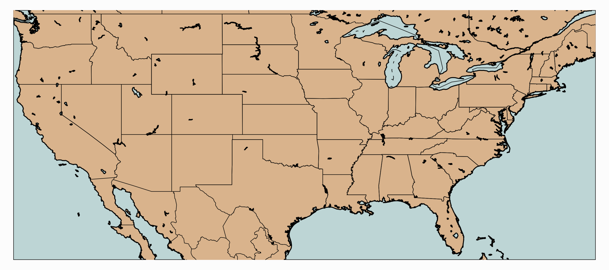
With the U.S. map plotted above, we can overlay the GOES-16 LST data using the latitude and longitude fixed grid outlined in the previous section.
A compilation of the previous sections and the current section has been assembled into one Python script, which produces GOES-16 LST data over the U.S. map. This code is given below, along with the data plot further below:
#!/usr/bin/python

from netCDF4 import Dataset
import matplotlib as mpl
mpl.use('TkAgg')
import matplotlib.pyplot as plt
from mpl_toolkits.basemap import Basemap, cm
import numpy as np
import os

def lat_lon_reproj(nc_folder):
    os.chdir(nc_folder)
    full_direc = os.listdir()
    nc_files = [ii for ii in full_direc if ii.endswith('.nc')]
    g16_data_file = nc_files[0] # select .nc file
    print(nc_files[0]) # print file name

    # designate dataset
    g16nc = Dataset(g16_data_file, 'r')
    var_names = [ii for ii in g16nc.variables]
    var_name = var_names[0]

    # GOES-R projection info and retrieving relevant constants
    proj_info = g16nc.variables['goes_imager_projection']
    lon_origin = proj_info.longitude_of_projection_origin
    H = proj_info.perspective_point_height+proj_info.semi_major_axis
    r_eq = proj_info.semi_major_axis
    r_pol = proj_info.semi_minor_axis

    # grid info
    lat_rad_1d = g16nc.variables['x'][:]
    lon_rad_1d = g16nc.variables['y'][:]

    # close file when finished
    g16nc.close()
    g16nc = None

    # create meshgrid filled with radian angles
    lat_rad,lon_rad = np.meshgrid(lat_rad_1d,lon_rad_1d)

    # lat/lon calc routine from satellite radian angle vectors

    lambda_0 = (lon_origin*np.pi)/180.0

    a_var = np.power(np.sin(lat_rad),2.0) + (np.power(np.cos(lat_rad),2.0)*(np.power(np.cos(lon_rad),2.0)+(((r_eq*r_eq)/(r_pol*r_pol))*np.power(np.sin(lon_rad),2.0))))
    b_var = -2.0*H*np.cos(lat_rad)*np.cos(lon_rad)
    c_var = (H**2.0)-(r_eq**2.0)

    r_s = (-1.0*b_var - np.sqrt((b_var**2)-(4.0*a_var*c_var)))/(2.0*a_var)

    s_x = r_s*np.cos(lat_rad)*np.cos(lon_rad)
    s_y = - r_s*np.sin(lat_rad)
    s_z = r_s*np.cos(lat_rad)*np.sin(lon_rad)

    # latitude and longitude projection for plotting data on traditional lat/lon maps
    lat = (180.0/np.pi)*(np.arctan(((r_eq*r_eq)/(r_pol*r_pol))*((s_z/np.sqrt(((H-s_x)*(H-s_x))+(s_y*s_y))))))
    lon = (lambda_0 - np.arctan(s_y/(H-s_x)))*(180.0/np.pi)

    os.chdir('../')

    return lon,lat

def data_grab(nc_folder,nc_indx):
    os.chdir(nc_folder)
    full_direc = os.listdir()
    nc_files = [ii for ii in full_direc if ii.endswith('.nc')]
    g16_data_file = nc_files[nc_indx] # select .nc file
    print(nc_files[nc_indx]) # print file name

    # designate dataset
    g16nc = Dataset(g16_data_file, 'r')
    var_names = [ii for ii in g16nc.variables]
    var_name = var_names[0]

    # data info
    data = g16nc.variables[var_name][:]
    data_units = g16nc.variables[var_name].units
    data_time_grab = ((g16nc.time_coverage_end).replace('T',' ')).replace('Z','')
    data_long_name = g16nc.variables[var_name].long_name

    # close file when finished
    g16nc.close()
    g16nc = None

    os.chdir('../')
    # print test coordinates
    print('{} N, {} W'.format(lat[318,1849],abs(lon[318,1849])))

    return data,data_units,data_time_grab,data_long_name,var_name

nc_folder = './GOES_files/' # define folder where .nc files are located
lon,lat = lat_lon_reproj(nc_folder)

file_indx = 10 # be sure to pick the correct file. Make sure the file is not too big either,
# some of the bands create large files (stick to band 7-16)

data,data_units,data_time_grab,data_long_name,var_name = data_grab(nc_folder,file_indx)
# main data grab from function above

data_bounds = np.where(data.data!=65535)
bbox = [np.min(lon[data_bounds]),
        np.min(lat[data_bounds]),
        np.max(lon[data_bounds]),
        np.max(lat[data_bounds])] # set bounds for plotting

# figure routine for visualization
fig = plt.figure(figsize=(9,4),dpi=200)

n_add = 0 # for zooming in and out
m = Basemap(llcrnrlon=bbox[0]-n_add,llcrnrlat=bbox[1]-n_add,urcrnrlon=bbox[2]+n_add,urcrnrlat=bbox[3]+n_add,resolution='i', projection='cyl')
m.fillcontinents(color='#d9b38c',lake_color='#bdd5d5',zorder=1) # continent colors
m.drawmapboundary(fill_color='#bdd5d5',zorder=0) # ocean color
m.drawcoastlines(linewidth=0.5)
m.drawcountries(linewidth=0.25)
m.drawstates(zorder=2)
m.pcolormesh(lon.data, lat.data, data, latlon=True,zorder=999) # plotting actual LST data
parallels = np.linspace(bbox[1],bbox[3],5.)
m.drawparallels(parallels,labels=[True,False,False,False],zorder=2,fontsize=8)
meridians = np.linspace(bbox[0],bbox[2],5.)
m.drawmeridians(meridians,labels=[False,False,False,True],zorder=1,fontsize=8)
cb = m.colorbar()

data_units = ((data_units.replace('-','^{-')).replace('1','1}')).replace('2','2}')
plt.rc('text', usetex=True)
cb.set_label(r'%s $ \left[ \mathrm \right] $'% (var_name,data_units))
plt.title(' on '.format(data_long_name,data_time_grab))
plt.tight_layout()

plt.savefig('goes_16_data_demo.png',dpi=200,facecolor=[252/255,252/255,252/255]) # uncomment to save figure
plt.show()
Above, we can see how the GOES-16 LST data sits atop the U.S. map, with latitude and longitude lines. We also have a colorbar representing the range of temperatures. Another observation that can be made is the warming with decreased latitude - which is expected as we approach the equator. Data sparseness is also a huge aspect of the LST data due to cloud interference. The LST product uses complex moisture information to ensure that the cited temperatures do not include interference from cloud - something could contaminate the true surface temperature approximation.
In this tutorial, the basics of retrieving and mapping satellite images was introduced using Python and several of its compatible libraries. The publicly-available GOES-16 satellite data makes imagery analysis accessible, and in our case, the land surface temperature (LST) product was used as an example for visualizing geographic data. The complexity of projections from space and geographic information makes the analysis of satellite data very complex, however, in this step-by-step series, I will explore some methods for comprehending data formats, understanding mapping, simple geographic statistics, and the application of satellite imagery in industry and research. This first entry is a simple introduction into the tools for data acquisition and visualization - in the next entry, actual satellite imagery analysis will be conducted with topics ranging from spatial trends, temporal trends, and algorithms.
See More in Python and GIS: