Geospatial Analysis Using QGIS and Open-Source Data
Geographic information systems (GIS) are powerful tools used by climatologists, health organizations, defense agencies, real-estate companies, and nearly all professions that rely on location-based data. Geographic data is often very cumbersome to analyze traditionally, which is why visualization tools are essential. Depending on the size and complexity of the data, several robust GIS softwares exist on the market from open-source (free) to paid subscriptions. Each software has its strengths and weaknesses, so depending on the application one software may be more effective than another. A few of the leading softwares are: GE Smallworld, Google Earth Pro, AutoCAD Map 3D, and Maptitude. QGIS is an open-source competitor to ArcGIS, which is arguably the industry leader in the GIS market, so for financial and ease-of-application reasons, QGIS is employed here. I will also cover four scales of geographic analysis: one at the city level (NYC), one at the state level (Washington State), one at the country level (U.S.A.), and one at the world level. The goal is to demonstrate the power and breadth of geographic information systems at any scale.
Shapefiles and Importing Data
I will be using two types of data for this analysis: shapefiles and comma separated values (csv). The raw data used in GIS is often comma separated; however, the second type, the shapefile, is used because it contains the geographic lines or polygons that create the shapes we often see in maps. In this tutorial, I will be using data from the following four sources:
Local (NYC) - https://data.cityofnewyork.us/Environment/Natural-Gas-Consumption-by-ZIP-Code-2010/uedp-fegm
State (WA) - https://data.wa.gov/Natural-Resources-Environment/Water-Quality-Index-Scores-1994-2013-from-The-WA-S/k5fe-2e4s
Country (U.S.A.) - https://catalog.data.gov/dataset/age-adjusted-death-rates-for-the-top-10-leading-causes-of-death-united-states-2013
Global (World) - https://data.worldbank.org/indicator/NY.GDP.MKTP.CD?year_high_desc=true
The datasets above may need some reformatting, so be sure to dig into the .csv files and get rid of multiple headers, replace NaN values, or chop the data into smaller sections depending on the extent of the desired analysis.
QGIS should be opened and a recent projects section should be shown (see below):

We want to start a new project, so we can just jump right into the menu bar on the left. Click on the 'V' icon on the left toolbar that says 'Add Vector Layer.' This is where you add your shapefile that you download for a particular location. In our case, it will be NYC.
Now, you should add your shapefile for the location. I used the zip code shapefile for NYC so we can investigate natural gas consumption in each zip code of the city. The zip code shapefile can be found here. Now, the following should be shown on the QGIS dashboard:


Now, we want to import the actual data from the OpenDataNYC website that contains the natural gas usage by zip code. We do this by clicking the comma on the left toolbar that says 'Add Delimited Text Layer.' After clicking the add delimited text layer and choosing the .csv file that contains the data, the following should be displayed:

The important thing to remember here is that we want to select 'No Geometry (attribute only table)' so that we can combine the data via zip code, and not by latitude or longitude. Thus, we now have a table of values for natural gas consumption and a map of the zip codes for New York City. We want to combine the two to create a joint distribution of data (csv file) that can be mapped by location (zip code shapefile). To do this, we have to double click the zip code shapefile on the layers panel. This should give us the following window:

Now, we select 'Joins' on the left toolbar and click the plus sign at the bottom of the window. Now, in the window that appears, you have to be sure that both zip codes are formatted the same way in each file (csv and shapefile). Then, we select those two zip code columns as the 'join field' and 'target field' for the join. From here, it is up to you what you select for which parameters are passed from the .csv file to the shapefile, but for simplicity's sake, we will leave those alone for now.
We should have a shapefile with an additional value. To test this, go to the top toolbar and select the arrow with the 'i' called 'identify features' and select one of the zip codes. You should see an additional few parameters at the end of the features list on the right toolbar.


At this point, the shapefile has taken on the values of the .csv file into each zip code. Now, one thing that can be done is to discretely divide the data into color-based values. To do this, we want to double click on the zip code shapefile again. This time, we want to select 'Style.'
From the 'Style' toolbar, select the top where it says 'Single Symbol.' We want to add some dynamism to this, so change it to 'Graduated.' This will make it easy to view the dynamics of the data.
In the 'Graduated' options of the 'Style' toolbar, select a column to analyze. I chose to analyze the Giga Joule Consumption. Then select classify, then Apply, and OK. This should give you the blue color ramped data shown below.
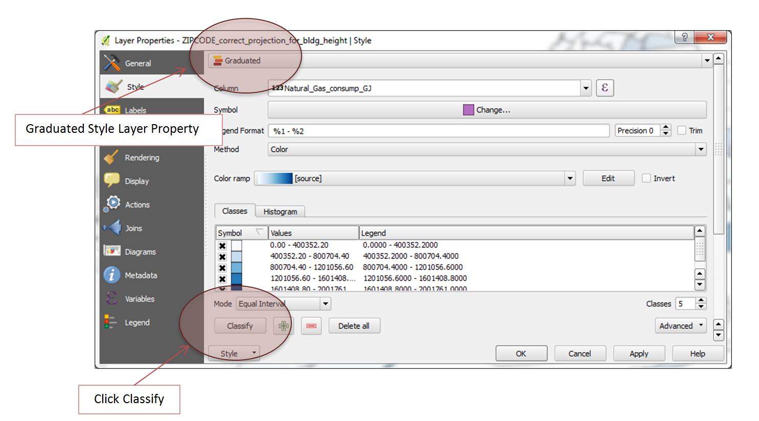

The above map in blue demonstrates the power of QGIS. The different colors show the variety of data: the darker the blue, the higher the consumption of natural gas in that zip code.
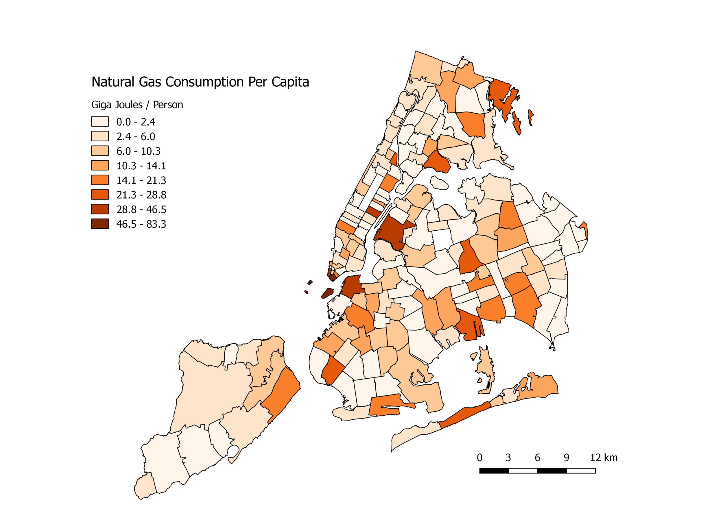
Below are two variations of the analysis above. The first plot (orange) is the natural gas consumption per capita. The second (in blue) is the consumption per area. Both demonstrate high concentrations in interesting areas, perhaps related to income. Both plots were derived using the method above and the same data. To achieve the results shown below, a slightly more complicated routine is used. The technique requires altering or creating new fields in the data and using minimal programming in QGIS. The method is explored below using the next scale of data, for Washington State.

Latitude and Longitude Raw Data, Creating New Fields, and More Intricate Analyses
Open a new QGIS project and import the Washington State Shapefile (find here). Now add the delimited file with the water quality data for Washington state (data here). Again, the data is slightly off-format, so you'll need to reformat the latitude and longitude values so that they can be recognized when imported into QGIS. This can be done by opening the data in Excel and separating the lat/lon vector into two columns. Upon reformat of the data, import the .csv but this time use the geometry of lat/lon columns instead of selecting the 'no geometry' option as done above. This will now distribute the data based on lat/lon coordinates, rather than zip codes as before. You should end up with something similar to what is shown below:

Currently, we have data points atop the shapefile of Washington State. We will not combine the shapefile and .csv data in this analysis, so the shapefile simply acts as a visual foundation for the water quality data. We will, however, alter the water quality data to produce more dynamic data representation. To start, we want to double click the water quality .csv data to view its layer properties.
Once in the layer properties of the data, click 'Single Symbol' again and change it to 'Graduated.' This time, we will be investigating graduated sizes, rather than colors. Where it says 'Method' select size. This will change the size of the bullets, rather than their colors, which would be hard to see.

You may also want to play around with the section below the Classify region to get the behavior of the layer just how you want it. You can alter the layer behavior (the behavior of the .csv data) to make the circles bigger, the behavior they exhibit when they overlap, etc. Below is my interpretation of the water quality data from 2013.

QGIS has a tool that also allows you to carry out mathematical routines. This can be useful for analyzing data and producing more meaningful results with the limited geospatial data that is available. Return again to the layer properties of the .csv data, but this time click on the 'Fields' tab.

From here, we want to select the 'Field Calculator' which should bring up the following window:

We now need to decide what information the new field will convey. I chose to average the 20 years of water quality data. However, this comes with a caveat - some of the data does not exist for all 20 years, so we end up with fewer points (because of NULL values). Now, there is a way around this, however, it's not something I want to cover in this limited tutorial. So, for now, we take what we can get and average the stations that have 20 years worth of data. To do this, you select the 20 variables from 'Fields and Values' and add them all together, then divide by 20. The result of this is shown below:

We're not necessarily looking for a trend here, and since there is no easily observable one, I will leave that analysis for another time (looking at population, nearby land use, etc.). That analysis would be a great project for someone interested in learning more about GIS and also producing meaningful results in the study of water quality. Perhaps a government entity interested in observing the changes that result in better/worse quality of water. For now, we will leave the Washington State map and proceed to analyze the contiguous United States data.
The third entry in this GIS tutorial will utilize the contiguous map of the United States of America (find the shapefile here). The data is entitled 'Age-Adjusted Death Rates For the Top 10 Leading Causes of Death' (find it here). The data spans from 1999 to 2015 and contains all 10 leading causes for each year, however, I chose only to investigate the deaths due to Heart Disease. Again, the csv file will need to be altered to format the data correctly. In this case, the dates need to be repositioned as columns in the csv file, rather than rows. After completing both of the analyses above, the contiguous U.S. analysis should be no issue. Below I combined the csv file and the shapefile, then used the graduated color method for visualizing the death rates.

Below, I subtracted the death rates for 2015 and 1999 to produce a difference plot. The more negative the data, the larger the change in heart disease-related deaths. Utah appears to be the state with the least progress made toward combating heart disease, while Louisiana appears to have the largest change the other way, it had the biggest decrease from 1999 to 2015 in heart disease-related deaths.

The final analysis is shown below for the whole world. The Gross Domestic Product is often a signature of the status of a country's economic market. Some data is missing because of different reasons, but the major countries are present as is their approximate domestic product. The leading countries are the U.S., China, Japan, and Germany. You can also see that much of Africa is on the lower end of the GDP. Europe is fairly high in ranking, while South America is in between, primarily due to Brazil and its place in the top 10.

Conclusion and Remarks
Geographic information systems are paramount in the investigation of location-based data. I investigated four very distinct types of geospatial data ranging from natural gas consumption, water quality index, all the way to disease-related deaths and GDP of the countries of the world. The power of GIS is reliant on the user, and I hope this short tutorial endowed some amount of competence in using one specific tool in the toolbox of geospatial analysis.
In the grand scheme of data analytics, the analyses shown here would be severely inadequate. I demonstrated simple mathematical techniques, without much description as to why. There is also often a certain amount of data filtering required, which was also not carried out here. Therefore, it is unwise to interpret this data too closely, but rather use it as a tool for completing your own investigation into patterns and trend in data whether it be for weather, disease mapping, spatial-dependent finance patterns, etc. When composing true analysis of data as sensitive as health trends, GDP, or water quality, there should always be a step-by-step description of where the data was taken from, how it was filtered, where there is data lacking; there should also be some statistical parameters calculated to ensure others that your conclusions are correct and justified. Moreover, I think this is a great starting point for anyone interested in GIS, and wants to start in the open-source region of the field.
See More in GIS: