Introduction To Capacitive MEMS Accelerometers and A Case Study On An Elevator
For many, acceleration is a concept that is taught in elementary physics but rarely matures past a discussion of gravity: think of a ball being thrown in the air, a pendulum swinging, or a cart rolling down an incline. In engineering, however, acceleration describes many of the complex phenomena at work in the aerospace, automotive, architectural, and seismological fields - just to name a few. A measurement or approximation of acceleration relates to the forces acting on a system, which can prevent disasters or loss of resources.
Mass-Spring Analogue
Consider the mass-spring system shown in Figure 1. Its differential equation is commonly written as:

where k is the spring constant, m is the mass of the object, and x is displacement. We can say that the second time derivative of the displacement is the acceleration, and we end up with the following:


Figure 1: Mass-spring system.
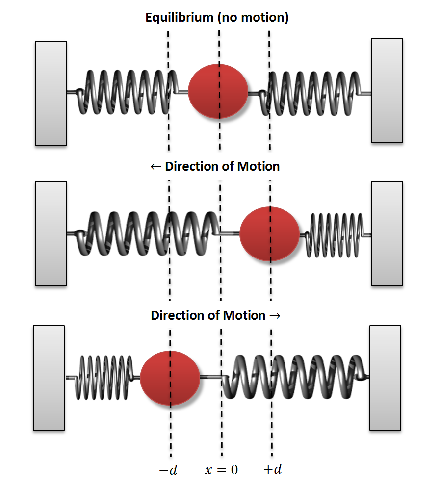
Figure 2: Double-walled mass spring system in a moving inertial reference frame. The walls are the primary while the ball moves in opposition to the
Now, imagine the double-walled mass-spring system shown in Figure 2. The only difference between the double-walled case and the simple mass-spring system above is a factor of two, assuming the springs are identical. It is also important to realize that the entire system moves, resulting in opposition of motion from the mass according to Newton's 2nd law, F = ma. Consequently, with prescribed mass and springs, the displacement of the mass is proportional to the accelerations experienced by the system. This problem is the first fundamental step toward creating what is called a capacitive accelerometer.
Capacitive MEMS Accelerometer
A micro-electromechanical system (MEMS) is a classification that describes microscopic devices made of both electrical and mechanical parts. A MEMS accelerometer is a device that measures acceleration by utilizing the techniques described above, but on a micro scale. The mass-spring system is the mechanical side of the MEMS device, and capacitance is the electrical portion. The capacitance of a parallel-plate capacitor is:

where C is capacitance, Q is charge, V is voltage, A is the area of the plate, ε is called the permitivity (constant), and d is the distance between the plates. Capcitance plays a key role in calculating the acceleration from the mass-spring system by measuring a change in voltage as the distance between two capacitive plates is changed.

Figure 3: Basic diagram of a parallel plate capacitor.
Imagine now a mass-spring system with the adjustments shown in the following image:

Figure 4: Simplified MEMS accelerometer in equilibrium.
One method for balancing the system above is to break down the electrical contributions using conservation of charge:

Furthermore, when the system is set into motion, the capacitances change and the setup can be explicitly modeled as follows:

Figure 5: Fully labeled diagram of a simplified MEMS accelerometer.
In Figure 5, the conservation of charge can be written as:

Again, the variable of interest is the displacement between the capacitors - this distance acts as the indicator of force applied to the mass, which will ultimately bestow information about the acceleration of the system. Utilizing the equations for capacitance, we have:

And finally, we can solve the above algebraic equation for the displacement of the mass:

At this point, it is easy to see how we can relate the knowns in the system to find acceleration:

This simple result endows us with immense power. The above equation states that with prescribed values of spring constants, movable mass, capacitor equilibrium separation distance, and an applied voltage, we can determine the acceleration of the system just by reading a voltage. This is an impressive conclusion despite the complex nature of the problem. It is a basis for understanding the capacitive MEMS accelerometers that are used and still built today, and it is also the foundation for the sensor used in the experiment below, which utilizes a capacitive MEMS accelerometer to measure forces and distance traveled in a commercial elevator.
[For more in-depth analysis and investigation of MEMS accelerometers see here, here, and here].
Accelerometer on an Elevator
On an elevator, weight fluctuates based on the acceleration of the vessel. If an elevator is accelerating upward, then a mass's weight will increase, and the opposite is true for a descending elevator. With all of this in mind, along with the knowledge of how a MEMS accelerometer works, I decided to verify Newton's 2nd law and the theory of gravitation (on earth's surface, at least). I used an ADXL345 (datasheet here, get one here), and interfaced with an Arduino and an iPhone using the HM-10 module and Bluetooth. That way, I was able to telemeter the acceleration data at roughly 17 samples/second in real time. The ADXL345 is capable of 100 samples/sec, so there was no worry of accuracy in time. However, the accuracy of the sensor itself proved to be less than ideal, along with positioning inaccuracies, as well as other shortcomings. These, however, will be discussed during the analysis section. The goal for this project was to analyze the maximum accelerations of a specific elevator (located in the Marshak Science Building on the campus of the City College of New York, see Figure 7), and examine the accuracy of numerical integration of a MEMS accelerometer to approximate distance traveled.

Figure 6: An elevator moving upward will increase a person's weight, while the opposite is true for a downward moving elevator.
Products from our shop useful for replicating this experiment:

The Raspberry Pi 4 Computer, Model B is the latest in the series of single-board computers (SBC) produced by the Raspberry Pi Foundation. The RPi 4 increased its processor speed, its GPU performance, memory (1GB, 2GB, 4B, 8GB options), and connectivity. The Raspberry Pi 4 computer continues to be an essential tool in the maker, programmer, and engineer communities. The Raspberry Pi 4 is capable of interfacing with a wide range of sensors, motors, actuators, and devices. The RPi 4 has the standard 40-pin header with general purpose input/outputs (GPIOs), Bluetooth and WiFi capabilities, HDMI output display abilities, and much more! Our site contains a variety of different tutorials in the categories of Python programming, data acquisition and analysis, motor control, internet of things (IoT), engineering, among others.
Included with the Raspberry Pi 4 Model B Computer:
1x Raspberry Pi 4 Model B Computer
Features of the Raspberry Pi 4 Model B Computer:
Broadcom BCM2711, Quad core Cortex-A72 (ARM v8) 64-bit SoC @ 1.5GHz
LPDDR4-3200 SDRAM (2GB, 4GB, 8GB depending on the model)
2.4 GHz and 5.0 GHz WiFi, Bluetooth 5.0, Bluetooth Low Energy (BLE)
Gigabit Ethernet
2x USB 3.0 ports; 2x USB 2.0 ports
Raspberry Pi standard 40-pin GPIO header (fully backwards compatible with previous boards)
2x micro-HDMI ports (up to 4K @60fps supported)
2-lane MIPI DSI display port, 2-lane MIPI CSI camera port
4-pole stereo audio and composite video port
H.265 (4kp60 decode), H264 (1080p60 decode, 1080p30 encode)
Micro-SD card slot for loading operating system and data storage
5V DC via USB-C connector, 5V DC via GPIO header (3A Recommended Supply)
Operating Temperature (Ambient): 0°C – 50°C
Raspberry Pi Peripherals:
6x UART, 6x I2C, 5x SPI, 1x SDIO, 1x DPI, 1x PCM, 2x PWM Channels, 3x GPCLK

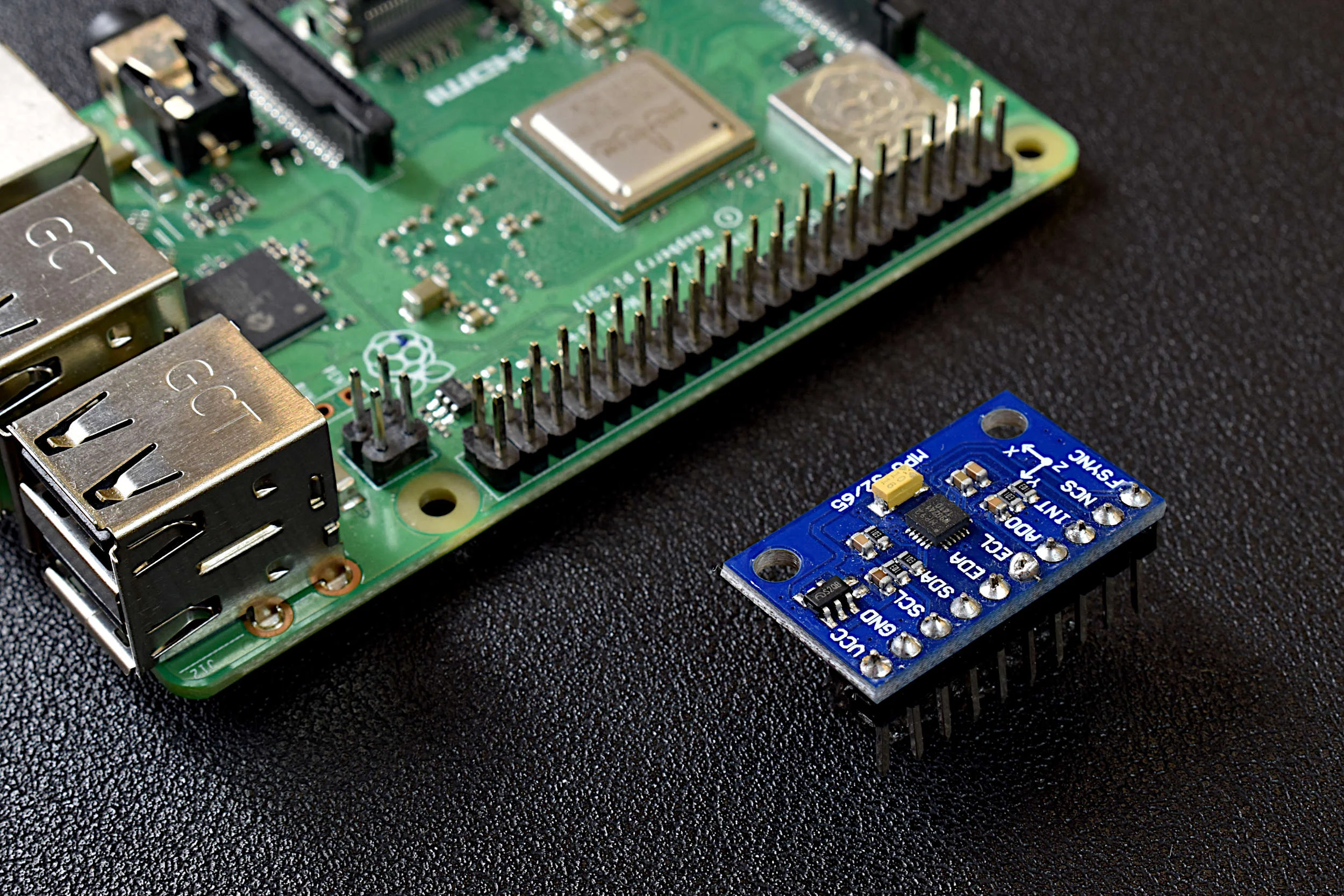
The MPU9250 is a 9 degree-of-freedom (9-DoF) inertial measurement unit (IMU). This incredible small profile sensor houses an accelerometer and gyroscope in the MPU6050 and a magnetometer in the AK8963. What an incredible combination for such a small device! The MPU9250 allows users to measure acceleration, angular velocity, magnetic inclination - all with the 2-wire I2C protocol.
Included in the MPU9250 Package:
1x MPU9250 IMU Board
10x Pin Header
Some Features of the MPU9250 IMU Board:
3-Axis Accelerometer (MPU6050)
±2g, ±4g, ±8g and ±16g with 16-bit ADC
~4000Hz Data Sample Rate
3-Axis Gyroscope (MPU6050)
±250, ±500, ±1000, and ±2000°/sec with 16-bit ADC
~8000Hz Max Data Sample Rate
3-Axis Magnetometer (AK8963)
±4800µT with 14-bit ADC
~ 8Hz-100Hz Data Sample Rate
I2C Communication Protocol
Low Power Consumption Options
Compatible with Arduino and Raspberry Pi
MPU9250 Datasheet

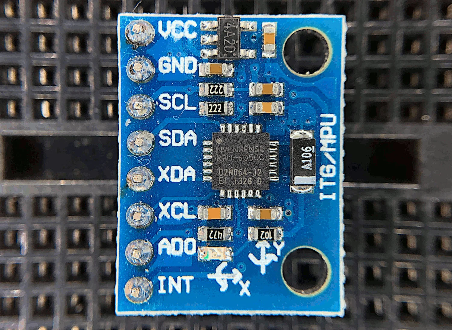
The MPU6050 is a 6-degree of freedom (DoF) inertial measurement unit (IMU) that measures acceleration in gravitational units (g) and angular velocity in degrees per second. The sensor has an onboard accelerometer and gyroscope that return 16-bit signed digital units, making the device fairly accurate for measuring rotation and accelerations in the three cardinal directions. The MPU6050 also measures temperature using an onboard temperature sensor.
The MPU6050 is fully compatible with Arduino and Raspberry Pi
Included in the MPU6050 sensor package:
MPU6050 Sensor
8-pin header
A tutorial using the MPU6050 IMU can be found on our site at: https://makersportal.com/blog/2019/8/17/arduino-mpu6050-high-frequency-accelerometer-and-gyroscope-data-saver
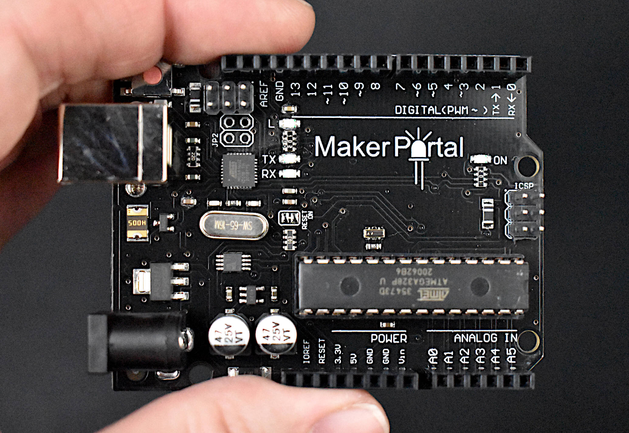
The Maker Portal Uno board is the centerpiece of many of the projects carried out in our maker spaces. The Uno board is capable of reading a wide range of sensors using analog-to-digital conversion, SPI, I2C, UART, and other common protocols. The Uno board can be used to control motors, OLED/LCD displays, and LEDs. The Arduino Uno board shown here is the official Maker Portal microcontroller, which we use in many of our projects!
Included in the Arduino Uno Package:
Maker Portal Arduino Uno Rev3 Board
Black USB Cable (1m in Length)
Specifications for Arduino Uno Rev3 Board:
ATmega328P chip with Arduino Bootloader
14 digital pins, 6 analog pins
10-bit analog-to-digital converter (ADC)
5V-12V Supply Tolerance
3.3V and 5.0V output pins
16 MHz clock
5 PWM pins, I2C support, SPI support , UART support
ATmega16U2 USB TTL, compatible with Linux, Windows, and Mac
Black Stylish Finish
Fully Integrated with Arduino IDE software
Methodology
The procedure for this experiment is simple:
Take continuous measurements of acceleration on an elevator
Ensure that multiple distances are measured - this means taking multiple rides in the elevator to different floors
Normalize the accelerometer data to account for gravity
Integrate the acceleration data over time to approximate instantaneous velocity
Integrate velocity data and sum to approximate displacement
Find maximum acceleration to investigate maximum forces
An example acceleration plot after application of a simple running mean filter is shown in Figure 8.

Figure 7: Marshak Science building where the acceleration measurements were made on several of the elevators. Image courtesy of www.rsdeng.com
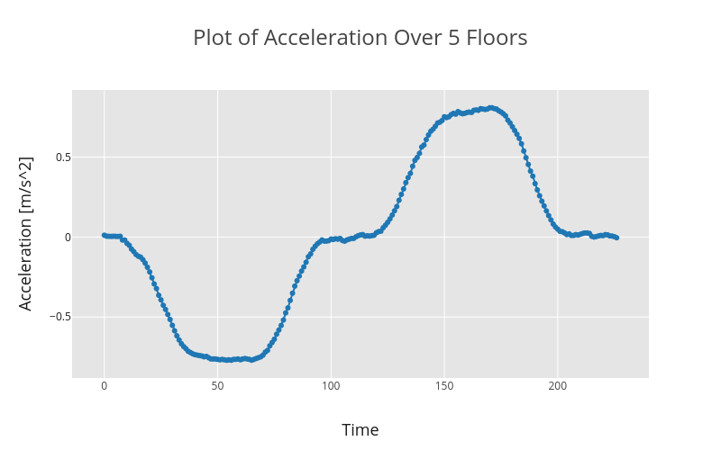
figure 8: Plot of Acceleration for one instance where 5 floors were traversed by an elevator. It is important to realize that the elevator accelerates in one direction to move upward or downward, and decelerates to stop and let people disembark. The above data was smoothed to eliminate erroneous data points. The accelerometer data was also normalized by gravity to account for only the acceleration of the body in its own frame of reference.
After acquiring the acceleration data and smoothing it with a simple high frequency filter, the effects of gravity need to be eliminated to ensure we only integrate the moving acceleration of the body (elevator). After approximating the influence of gravity from the steady-state of the sensor, I numerically integrated the discrete data using the following trapezoidal method:


After carrying out the above integration, we now have instantaneous velocity data and with instantaneous velocity, displacement can easily be calculated. At this point, the velocity can be integrated via the same procedure, or the displacement can be obtained from the sum of the velocities multiplied by the time spacing between them - either one should be a good approximation for this particular case.

Finally, we arrive at a displacement. I carried out several of these calculations of displacement for multiple traverses between building floors in the Marshak Science Building (Figure 7), and I arrived at a plot of floors traversed vs. distance calculated, as shown in Figure 9.
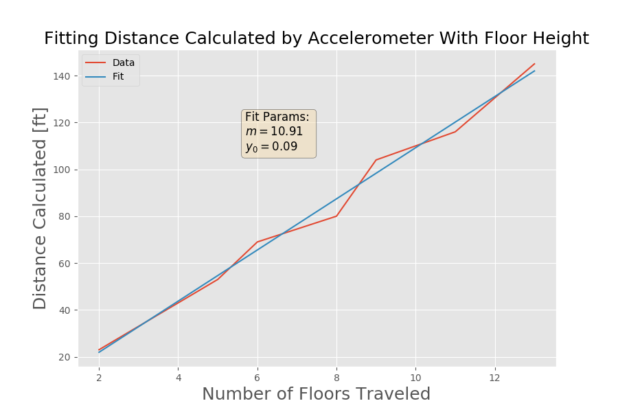
Figure 9: Plot of number of floors traversed vs. distance calculated. This plot contains the raw approximations with the linear fit. It can be seen that the approximate height of each floor is about 11 ft. This makes perfect sense considering the height of the building (166 ft). There are 13 regular floors, plug roughly two others to get to the roof. Therefore, if the building is approximated to be 15 stories, then 10.91 x 15 = 163.7 ft. This appears to be a decent approximation, considering the level of accuracy of the sensor.
The fit shown in Figure 9 concludes that the height of each floor is approximately 10.9 ft. This appears to be a fairly accurate prediction of the height of this particular building, due to the prior knowledge of its height (166 ft). There are 13 stories in the building accessible by elevator, and 2 additional floors to arrive at the roof. Therefore, the approximate building height from these calculations heeds 163.7 ft, which is within 2% of the actual building height.


Where a' is the fluctuating acceleration after gravity is subtracted. The negative sign states that if the fluctuating acceleration is greater than zero, then the body is traveling in the same direction as gravity, resulting in a net loss of weight; and for a negative fluctuating acceleration, the body is traveling against gravity, resulting in a net gain of weight. This is a fascinating study, and one that I'm sure manufacturers have to account for in fabrication of elevators and other transportation machinery. The experiments using an Arduino board, Bluetooth communication, Python for post-processing, and some elementary physics proved to be highly accurate and elucidatory for a classic physics and engineering problem that many of us take for granted.
Python Code
POLYFIT FOR FLOOR HEIGHT LINEAR REGRESSION
# polyfitting for floor height
#
#
import matplotlib as mpl
mpl.use('tkagg')
import numpy as np
import matplotlib.pyplot as plt
##plt.style.use('ggplot')
plt.style.use('ggplot')


bldg_floors = [2,5,6,8,9,11,13]
bldg_heights = [23,53,69,80,104,116,145]

poly_fit = np.polyfit(bldg_floors,bldg_heights,1)
poly_map = np.poly1d(poly_fit)


plt1,ax = plt.subplots(1,figsize=(9,6),dpi=100)

#plt.figure(figsize=(9,6),dpi=100)

ax.plot(bldg_floors,bldg_heights,label='Data')
plt.plot(bldg_floors,poly_map(bldg_floors),label='Fit')
plt.title('Fitting Distance Calculated by Accelerometer With Floor Height',fontsize=18)
plt.xlabel('Number of Floors Traveled',fontsize=18)
plt.ylabel('Distance Calculated [ft]',fontsize=18)
plt.legend()


txtstr_fit = 'Fit Params: \n$m = %0.2f$\n$y_0 = %0.2f$'%(poly_fit[0],poly_fit[1])
props = dict(boxstyle = 'round',facecolor='wheat',alpha=0.5,ec='k')
plt.text(0.35,0.8,txtstr_fit,transform=ax.transAxes,fontsize=12,\
         verticalalignment='top',bbox=props)

plt.show()
plt.savefig('bldg_fitting.png',transparent=True,dpi=400)
IMPORTING, FILTERING, AND PLOTTING CSV ACCELEROMETER DATA
import plotly.plotly as py
import plotly.graph_objs as go
import csv
import numpy as np
from scipy import integrate
from datetime import datetime

dat_val = np.array([])
time_vec = np.array([])
file_name = 'G_to_13th_fl'
with open(file_name+'.csv') as csvfile:
    reader = csv.DictReader(csvfile)
    for row in reader:
        (t_hr,t_min) = (row['Date']).split('+')
        t_sec = datetime.strptime(t_hr,'%Y-%m-%d %H:%M:%S ')
        time_vec = np.append(time_vec,t_sec)
        dat_val = np.append(dat_val,float(row['Data Reading']))
##        time_mon.append(int(row['Interval_End_Time'][0]))
##        time_vec.append(int(t_hr))

n_start =0
n_end = 404#len(dat_val)
interv_to_int = (np.linspace(n_start,n_end,n_end-n_start+1,dtype=int))
interv_to_int = interv_to_int[0:len(interv_to_int)-2]

dat_val = dat_val[interv_to_int]-np.mean(dat_val[0:15])

conv_size = 10

dat_val = np.convolve(dat_val,np.ones(conv_size),'same')/conv_size


##dat_val = dat_val+9.95
time_vec = time_vec[interv_to_int]
delta_x = np.mean(np.diff(time_vec))
dx = delta_x.total_seconds()
vel = integrate.cumtrapz(dat_val)*dx
dist_approx = np.trapz(vel)*dx
print("Approximate Distance Traveled: "+str(dist_approx*3.28084))

##time_vec = datetime.strptime(time_vec,'%Y-%m-%d %H:%M:%S')
time_vec = np.linspace(0,len(time_vec),len(time_vec)+1)
time_vec = time_vec[0:len(time_vec)-1]
trace = go.Scatter(
    x = time_vec,
    y = dat_val,
    name = 'Plot of Ground to 13th Floor Acceleration in y-direction',
    mode='lines+markers'
    )

layout = go.Layout(
    paper_bgcolor = 'rgb(255,255,255)',
    plot_bgcolor='rgb(229,229,229)',
    width = 800,
    title = 'Plot of Ground to 13th Floor Acceleration in y-direction',
    titlefont = dict(
        size=24
        ),
    xaxis = dict(
        title='Time',
        titlefont=dict(
            size = 18,
            color='rgb(0.1,0.1,0.1)'
            ),
        gridcolor='rgb(255,255,255)',
        zeroline = False,
##        range=[min(dat_val),max(dat_val)]
        ),
    yaxis = dict(
        title='Acceleration [m/s^2]',
        titlefont=dict(
            size = 18,
            color='rgb(0.1,0.1,0.1)'
            ),
        tickfont = dict(
            color = 'rgb(0.1,0.1,0.1)'
            ),
        gridcolor='rgb(255,255,255)',
        zeroline = False
        )
    )


fig = go.Figure(data=[trace],layout=layout)
plot_url = py.plot(fig,filename=file_name,auto_open=False)
See More in Raspberry Pi and Inertial Measurement Units:
Related Products:
The MPU9250 is a 9 degree-of-freedom (9-DoF) inertial measurement unit (IMU). This incredible small profile sensor houses an accelerometer and gyroscope in the MPU6050 and a magnetometer in the AK8963. What an incredible combination for such a small device! The MPU9250 allows users to measure acceleration, angular velocity, magnetic inclination - all with the 2-wire I2C protocol.
Included in the MPU9250 Package:
1x MPU9250 IMU Board
10x Pin Header
Some Features of the MPU9250 IMU Board:
3-Axis Accelerometer (MPU6050)
±2g, ±4g, ±8g and ±16g with 16-bit ADC
~4000Hz Data Sample Rate
3-Axis Gyroscope (MPU6050)
±250, ±500, ±1000, and ±2000°/sec with 16-bit ADC
~8000Hz Max Data Sample Rate
3-Axis Magnetometer (AK8963)
±4800µT with 14-bit ADC
~ 8Hz-100Hz Data Sample Rate
I2C Communication Protocol
Low Power Consumption Options
Compatible with Arduino and Raspberry Pi
MPU9250 Datasheet
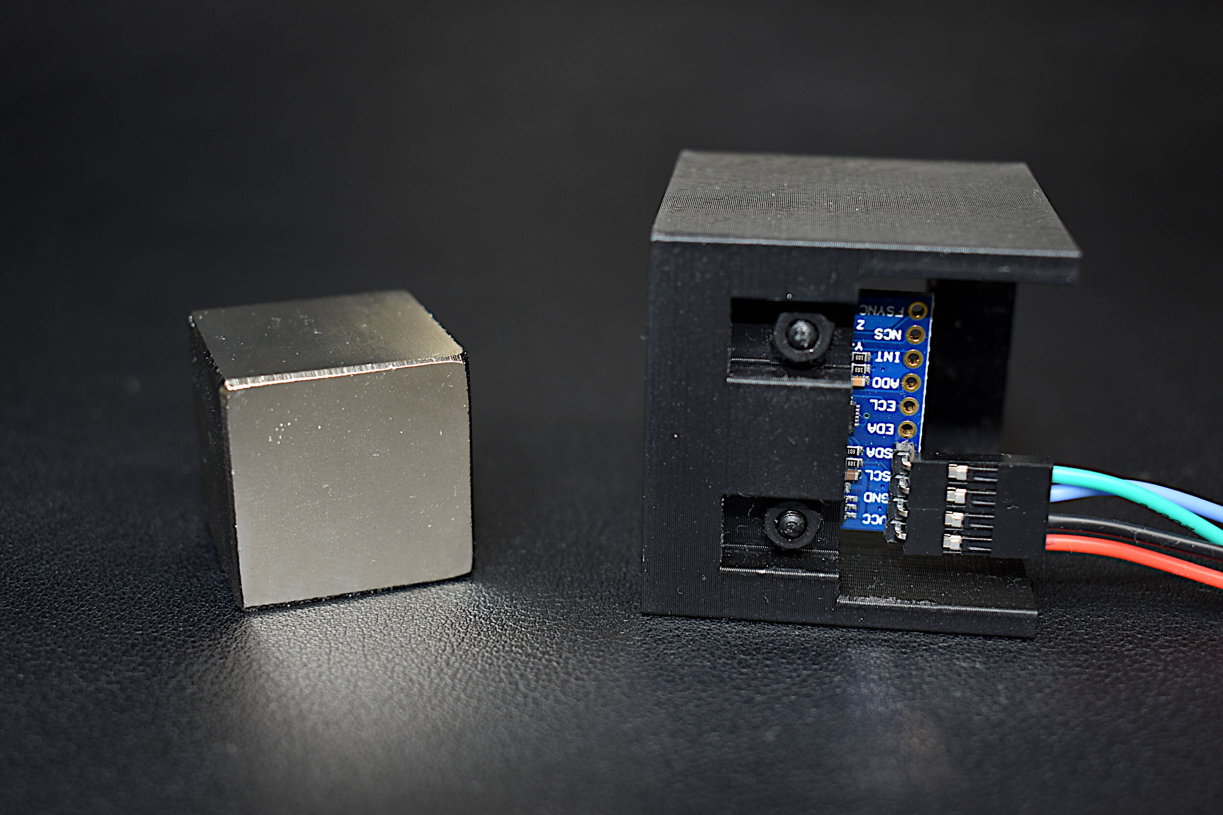
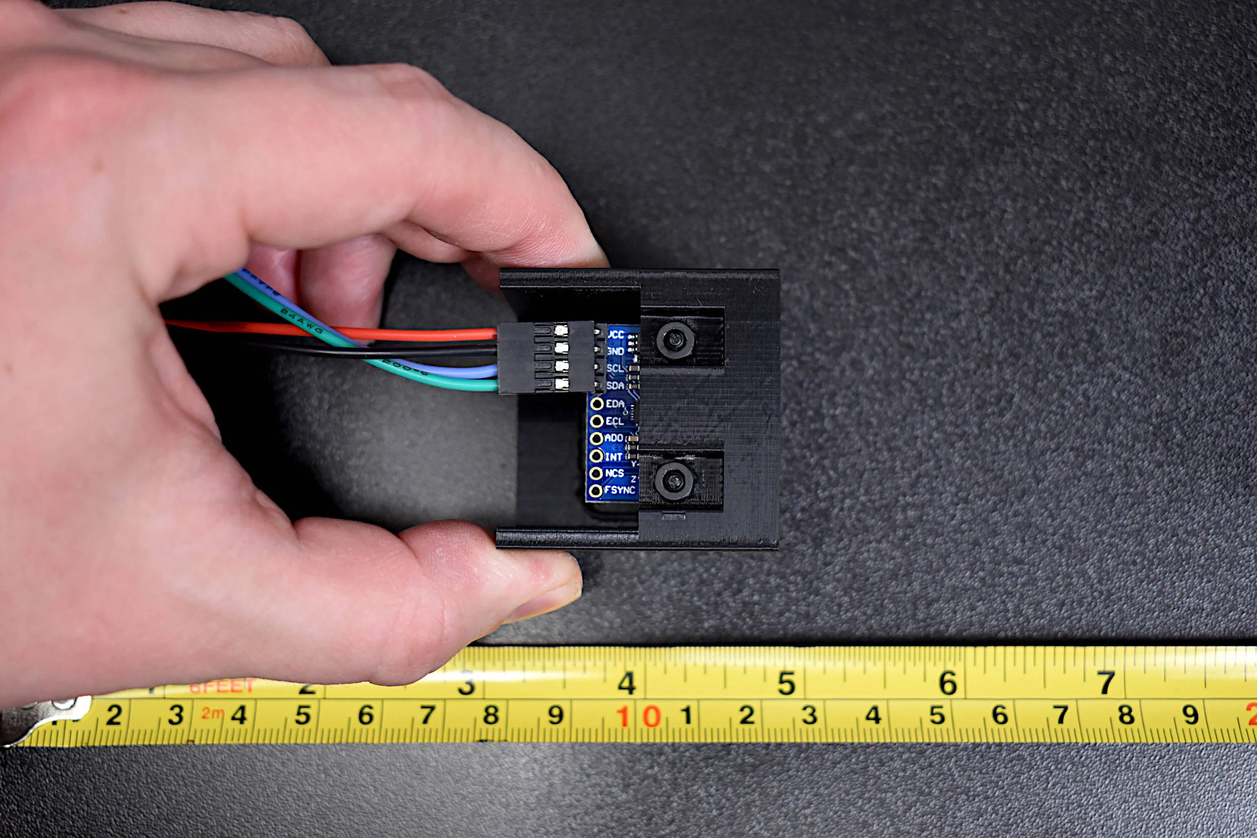
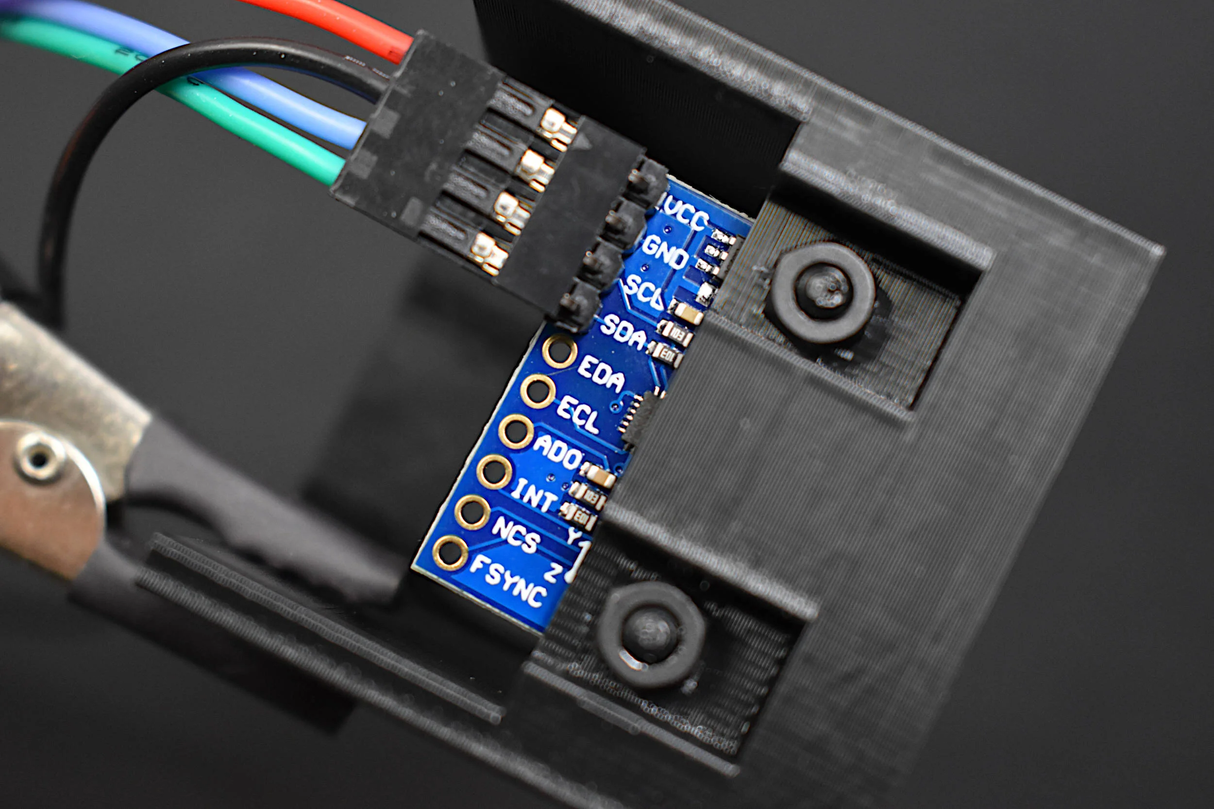
The calibration of an inertial measurement unit (IMU) is made simple in this kit by combining an MPU9250 sensor with a 3D-printed cube. The gyroscope contained within the MPU9250 can be calibrated under steady conditions. Similarly, the accelerometer can be calibrated by rotating each axis in the direction of gravity. Lastly, the magnetometer can be calibrated by rotating the block 360 degrees around each axis. The calibration block is specially designed for rotation and calibration of all nine degrees-of-freedom (9-DoF) available to the MPU9250.
See the IMU Calibration Series Tutorials: Part I, Part II, Part III
Included in the IMU Calibration Block Kit:
1x Calibration Block (40mm Cube)
1x MPU9250 Inertial Measurement Unit
2x Nylon Screws, 2x Nylon Nut
1x 4-Pin Dupont Connection Wire (24-AWG, 1 meter)
2x 10-Pin Header
PLA Material and Nylon Screws are used to Prevent Ferritic Interference with Magnetometer
Features of the IMU Calibration Block:
Designed for Calibration of all 9-DoF of the IMU
Holes for attaching MPU9250
Smooth to allow for rotation
90-degree edges for proper calibration in each direction
Sleek black design
Features of the MPU9250 IMU:
Easily attachable to the calibration block
Accelerometer/Gyroscope (MPU6050)
Magnetometer (AK8963)
Fast sample rates ~100Hz (Magnetometer), 1-8kHz (Accel/Gyro)
16-bit Analog-to-Digital Conversion for each of the 9-DoF
I2C Communication Protocol
Low Power Consumption
Compatible with Arduino and Raspberry Pi
MPU9250 Datasheet
3-Axis Accelerometer (MPU6050)
±2g, ±4g, ±8g and ±16g with 16-bit ADC
~4000Hz Data Sample Rate
3-Axis Gyroscope (MPU6050)
±250, ±500, ±1000, and ±2000°/sec with 16-bit ADC
~8000Hz Max Data Sample Rate
3-Axis Magnetometer (AK8963)
±4800µT with 14-bit ADC
~ 8-100Hz Data Sample Rate
The MPU6050 is a 6-degree of freedom (DoF) inertial measurement unit (IMU) that measures acceleration in gravitational units (g) and angular velocity in degrees per second. The sensor has an onboard accelerometer and gyroscope that return 16-bit signed digital units, making the device fairly accurate for measuring rotation and accelerations in the three cardinal directions. The MPU6050 also measures temperature using an onboard temperature sensor.
The MPU6050 is fully compatible with Arduino and Raspberry Pi
Included in the MPU6050 sensor package:
MPU6050 Sensor
8-pin header
A tutorial using the MPU6050 IMU can be found on our site at: https://makersportal.com/blog/2019/8/17/arduino-mpu6050-high-frequency-accelerometer-and-gyroscope-data-saver
The Raspberry Pi 4 Computer, Model B is the latest in the series of single-board computers (SBC) produced by the Raspberry Pi Foundation. The RPi 4 increased its processor speed, its GPU performance, memory (1GB, 2GB, 4B, 8GB options), and connectivity. The Raspberry Pi 4 computer continues to be an essential tool in the maker, programmer, and engineer communities. The Raspberry Pi 4 is capable of interfacing with a wide range of sensors, motors, actuators, and devices. The RPi 4 has the standard 40-pin header with general purpose input/outputs (GPIOs), Bluetooth and WiFi capabilities, HDMI output display abilities, and much more! Our site contains a variety of different tutorials in the categories of Python programming, data acquisition and analysis, motor control, internet of things (IoT), engineering, among others.
Included with the Raspberry Pi 4 Model B Computer:
1x Raspberry Pi 4 Model B Computer
Features of the Raspberry Pi 4 Model B Computer:
Broadcom BCM2711, Quad core Cortex-A72 (ARM v8) 64-bit SoC @ 1.5GHz
LPDDR4-3200 SDRAM (2GB, 4GB, 8GB depending on the model)
2.4 GHz and 5.0 GHz WiFi, Bluetooth 5.0, Bluetooth Low Energy (BLE)
Gigabit Ethernet
2x USB 3.0 ports; 2x USB 2.0 ports
Raspberry Pi standard 40-pin GPIO header (fully backwards compatible with previous boards)
2x micro-HDMI ports (up to 4K @60fps supported)
2-lane MIPI DSI display port, 2-lane MIPI CSI camera port
4-pole stereo audio and composite video port
H.265 (4kp60 decode), H264 (1080p60 decode, 1080p30 encode)
Micro-SD card slot for loading operating system and data storage
5V DC via USB-C connector, 5V DC via GPIO header (3A Recommended Supply)
Operating Temperature (Ambient): 0°C – 50°C
Raspberry Pi Peripherals:
6x UART, 6x I2C, 5x SPI, 1x SDIO, 1x DPI, 1x PCM, 2x PWM Channels, 3x GPCLK