Satellite Imagery Analysis in Python Part II: GOES-16 Land Surface Temperature (LST) Manipulation
This is the second entry in the satellite imagery analysis in Python. For part I, click here.
For part II, the focus shifts from the introduction of file formats and libraries to the geospatial analysis of satellite images. Python will again be used, along with many of its libraries. Land Surface Temperature will again be used as the data information, along with shapefiles used for geometric boundary setting, as well as information about buildings and land cover produced by local governments - all of which are used in meteorological and weather research and analyses.
A shapefile is a file format used to identify geographic boundaries and attributes of given geometries on earth [read more here]. Shapefiles are often used to quantify statistically significant information associated with rural, suburban, and urban areas. As an introduction to statistical analysis of satellite imagery, I will use a publicly-available shapefile of New York City (NYC). The shapefile can be downloaded at the following link:
https://data.cityofnewyork.us/api/geospatial/tqmj-j8zm?method=export&format=Shapefile
After downloading the file, unzip it and place it in the local Python script folder. The NYC shapefile can be plotted using similar Python Basemap methods introduced in the first entry in this satellite series. A code example is shown below, along with the sample output plot:
#!/usr/bin/python

import matplotlib as mpl
mpl.use('TkAgg')
import matplotlib.pyplot as plt
from mpl_toolkits.basemap import Basemap
import numpy as np

# create dummy figure for reading shapefile and setting boundaries
fig1 = plt.figure()
m1 = Basemap()
shp = m1.readshapefile('./Borough Boundaries/geo_export_23efe675-9411-42f6-812b-8775e2ba657d', 'nyc_shapefile')
plt.close(fig1) # close dummy figure
m1 = ()

# plotting actual shapefile
bbox = [shp[2][0],shp[2][1],shp[3][0],shp[3][1]]
fig,ax = plt.subplots(figsize=(14,8))
m = Basemap(llcrnrlon=bbox[0],llcrnrlat=bbox[1],urcrnrlon=bbox[2],
            urcrnrlat=bbox[3],resolution='i', projection='cyl')
m.readshapefile('./Borough Boundaries/geo_export_23efe675-9411-42f6-812b-8775e2ba657d',
                'nyc_shapefile',zorder=0)
parallels = np.linspace(bbox[1],bbox[3],5.) # latitudes
m.drawparallels(parallels,labels=[True,False,False,False],fontsize=12)
meridians = np.linspace(bbox[0],bbox[2],5.) # longitudes
m.drawmeridians(meridians,labels=[False,False,False,True],fontsize=12)

plt.savefig('nyc_shapefile_plain.png',dpi=200,facecolor=[252/255,252/255,252/255]) # uncomment to save figure
plt.show()

We will use this shapefile to quantify variation of land surface temperature over each borough of New York City. The shapefile contains information about each borough, which we can analyze using the following method:
m.nyc_shapefile_info
If we print out the first polygon in the shapefile it gives the following:
{'boro_code': 2.0, 'boro_name': 'Bronx', 'shape_area': 1186612476.97, 'shape_leng': 462958.186921, 'RINGNUM': 1, 'SHAPENUM': 1}
Where we can see the borough code and borough name, along with the area and length of the shape. We can use the borough codes to color each borough of the city:
#!/usr/bin/python

from netCDF4 import Dataset
import matplotlib as mpl
mpl.use('TkAgg')
import matplotlib.pyplot as plt
from mpl_toolkits.basemap import Basemap
from matplotlib.patches import Polygon
from matplotlib.collections import PatchCollection
from matplotlib.patches import PathPatch
import numpy as np

# create dummy figure for reading shapefile and setting boundaries
fig1 = plt.figure()
m1 = Basemap()
shp = m1.readshapefile('./Borough Boundaries/geo_export_23efe675-9411-42f6-812b-8775e2ba657d', 'nyc_shapefile')
plt.close(fig1) # close dummy figure
m1 = ()

# plotting actual shapefile
bbox = [shp[2][0],shp[2][1],shp[3][0],shp[3][1]]
fig,ax = plt.subplots(figsize=(14,8))
##ax.set_axis_off()
m = Basemap(llcrnrlon=bbox[0],llcrnrlat=bbox[1],urcrnrlon=bbox[2],
            urcrnrlat=bbox[3],resolution='i', projection='cyl')
m.readshapefile('./Borough Boundaries/geo_export_23efe675-9411-42f6-812b-8775e2ba657d', 'nyc_shapefile')
m.drawmapboundary(fill_color='#bdd5d5')
parallels = np.linspace(bbox[1],bbox[3],5.) # latitudes
m.drawparallels(parallels,labels=[True,False,False,False],fontsize=12)
meridians = np.linspace(bbox[0],bbox[2],5.) # longitudes
m.drawmeridians(meridians,labels=[False,False,False,True],fontsize=12)
plt.tight_layout()

boro_array = []
for ii in m.nyc_shapefile_info:
    boro_array.append(ii['boro_code'])

boro_unique = np.unique(boro_array)
colors = ['r','b','k','g','m']
for boro_iter in range(0,len(boro_unique)):
    patches   = []
    for ii,jj in zip(m.nyc_shapefile_info, m.nyc_shapefile):
        if ii['boro_code']==boro_unique[boro_iter]:
            patches.append(Polygon(np.array(jj),True))

    ax.add_collection(PatchCollection(patches, facecolor= colors[boro_iter], edgecolor='k', linewidths=1., zorder=2))

plt.savefig('nyc_shapefile_colors.png',dpi=200,facecolor=[252/255,252/255,252/255]) # uncomment to save figure
plt.show()

Since we are only interested in a small region for analysis (NYC), we can use the shapefile of the city to clip the boundaries of data and minimize the amount of processing needed. The code below is a continuation of the codes outline above, with the addition of corner calculations that find the indices of the lower-left, upper-left, lower-right, and upper-right corners of the LST file. This will allow us to clip the full 1500x2500 data file down to a much smaller size for more efficient processing.
#!/usr/bin/python

from netCDF4 import Dataset
import os,ogr
import matplotlib as mpl
mpl.use('TkAgg')
import matplotlib.pyplot as plt
from mpl_toolkits.basemap import Basemap
from matplotlib.patches import Polygon
from matplotlib.collections import PatchCollection
from matplotlib.patches import PathPatch
import numpy as np

def lat_lon_reproj(nc_folder):
    os.chdir(nc_folder)
    full_direc = os.listdir()
    nc_files = [ii for ii in full_direc if ii.endswith('.nc')]
    g16_data_file = nc_files[0] # select .nc file
    print(nc_files[0]) # print file name

    # designate dataset
    g16nc = Dataset(g16_data_file, 'r')
    var_names = [ii for ii in g16nc.variables]
    var_name = var_names[0]

    # GOES-R projection info and retrieving relevant constants
    proj_info = g16nc.variables['goes_imager_projection']
    lon_origin = proj_info.longitude_of_projection_origin
    H = proj_info.perspective_point_height+proj_info.semi_major_axis
    r_eq = proj_info.semi_major_axis
    r_pol = proj_info.semi_minor_axis

    # grid info
    lat_rad_1d = g16nc.variables['x'][:]
    lon_rad_1d = g16nc.variables['y'][:]

    # close file when finished
    g16nc.close()
    g16nc = None

    # create meshgrid filled with radian angles
    lat_rad,lon_rad = np.meshgrid(lat_rad_1d,lon_rad_1d)

    # lat/lon calc routine from satellite radian angle vectors

    lambda_0 = (lon_origin*np.pi)/180.0

    a_var = np.power(np.sin(lat_rad),2.0) + (np.power(np.cos(lat_rad),2.0)*\
                                             (np.power(np.cos(lon_rad),2.0)+\
                                              (((r_eq*r_eq)/(r_pol*r_pol))*\
                                               np.power(np.sin(lon_rad),2.0))))
    b_var = -2.0*H*np.cos(lat_rad)*np.cos(lon_rad)
    c_var = (H**2.0)-(r_eq**2.0)

    r_s = (-1.0*b_var - np.sqrt((b_var**2)-(4.0*a_var*c_var)))/(2.0*a_var)

    s_x = r_s*np.cos(lat_rad)*np.cos(lon_rad)
    s_y = - r_s*np.sin(lat_rad)
    s_z = r_s*np.cos(lat_rad)*np.sin(lon_rad)

    # latitude and longitude projection for plotting data on traditional lat/lon maps
    lat = (180.0/np.pi)*(np.arctan(((r_eq*r_eq)/(r_pol*r_pol))*\
                                   ((s_z/np.sqrt(((H-s_x)*(H-s_x))+(s_y*s_y))))))
    lon = (lambda_0 - np.arctan(s_y/(H-s_x)))*(180.0/np.pi)

    os.chdir('../')

    return lon,lat

def data_grab(nc_folder,nc_indx):
    os.chdir(nc_folder)
    full_direc = os.listdir()
    nc_files = [ii for ii in full_direc if ii.endswith('.nc')]
    g16_data_file = nc_files[nc_indx] # select .nc file
    print(nc_files[nc_indx]) # print file name

    # designate dataset
    g16nc = Dataset(g16_data_file, 'r')
    var_names = [ii for ii in g16nc.variables]
    var_name = var_names[0]

    # data info
    data = g16nc.variables[var_name][:]
    data_units = g16nc.variables[var_name].units
    data_time_grab = ((g16nc.time_coverage_end).replace('T',' ')).replace('Z','')
    data_long_name = g16nc.variables[var_name].long_name

    # close file when finished
    g16nc.close()
    g16nc = None

    os.chdir('../')
    # print test coordinates
    print('{} N, {} W'.format(lat[318,1849],abs(lon[318,1849])))

    return data,data_units,data_time_grab,data_long_name,var_name

##################
# create dummy figure for reading shapefile and setting boundaries
##################

fig1 = plt.figure()
m1 = Basemap()
shp = m1.readshapefile('./Borough Boundaries/geo_export_23efe675-9411-42f6-812b-8775e2ba657d',
                       'nyc_shapefile')
plt.close(fig1) # close dummy figure
m1 = ()

##################
# plotting actual shapefile
##################

bbox = [shp[2][0],shp[2][1],shp[3][0],shp[3][1]]
fig,ax = plt.subplots(figsize=(14,8))
m = Basemap(llcrnrlon=bbox[0],llcrnrlat=bbox[1],urcrnrlon=bbox[2],
            urcrnrlat=bbox[3],resolution='i', projection='cyl')
m.readshapefile('./Borough Boundaries/geo_export_23efe675-9411-42f6-812b-8775e2ba657d',
                'nyc_shapefile')
m.drawmapboundary(fill_color='#bdd5d5')
parallels = np.linspace(bbox[1],bbox[3],5.) # latitudes
m.drawparallels(parallels,labels=[True,False,False,False],fontsize=12)
meridians = np.linspace(bbox[0],bbox[2],5.) # longitudes
m.drawmeridians(meridians,labels=[False,False,False,True],fontsize=12)

##################
# finding boroughs and isolating them for shading in colors
##################

boro_array = []
for ii in m.nyc_shapefile_info:
    boro_array.append(ii['boro_code'])

boro_unique = np.unique(boro_array)
colors = ['r','b','k','g','m']
for boro_iter in range(0,len(boro_unique)):
    patches   = []
    for ii,jj in zip(m.nyc_shapefile_info, m.nyc_shapefile):
        if ii['boro_code']==boro_unique[boro_iter]:
            patches.append(Polygon(np.array(jj),True))

    ax.add_collection(PatchCollection(patches, facecolor= colors[boro_iter],
                                      edgecolor='k', linewidths=1., zorder=2))

##################
# GOES-16 LST section
##################

nc_folder = './GOES_files/' # define folder where .nc files are located
lon,lat = lat_lon_reproj(nc_folder)

file_indx = 10 # be sure to pick the correct file. Make sure the file is not too big either,
# some of the bands create large files (stick to band 7-16)

data,data_units,data_time_grab,data_long_name,var_name = data_grab(nc_folder,file_indx)

##################
# clipping lat/lon/data vectors to shapefile bounds
##################
# lower-left corner
llcrnr_loc_x = np.ma.argmin(np.ma.min(np.abs(np.ma.subtract(lon,bbox[0]))+\
                                      np.abs(np.ma.subtract(lat,bbox[1])),0))
llcrnr_loc = (np.ma.argmin(np.abs(np.ma.subtract(lon,bbox[0]))+\
                           np.abs(np.ma.subtract(lat,bbox[1])),0))[llcrnr_loc_x]
# upper-left corner
ulcrnr_loc_x = np.ma.argmin(np.ma.min(np.abs(np.ma.subtract(lon,bbox[0]))+\
                                      np.abs(np.ma.subtract(lat,bbox[3])),0))
ulcrnr_loc = (np.ma.argmin(np.abs(np.ma.subtract(lon,bbox[0]))+\
                           np.abs(np.ma.subtract(lat,bbox[3])),0))[ulcrnr_loc_x]
# lower-right corner
lrcrnr_loc_x = np.ma.argmin(np.ma.min(np.abs(np.ma.subtract(lon,bbox[2]))+\
                                      np.abs(np.ma.subtract(lat,bbox[1])),0))
lrcrnr_loc = (np.ma.argmin(np.abs(np.ma.subtract(lon,bbox[2]))+\
                           np.abs(np.ma.subtract(lat,bbox[1])),0))[lrcrnr_loc_x]
# upper-right corner
urcrnr_loc_x = np.ma.argmin(np.ma.min(np.abs(np.ma.subtract(lon,bbox[2]))+\
                                      np.abs(np.ma.subtract(lat,bbox[3])),0))
urcrnr_loc = (np.ma.argmin(np.abs(np.ma.subtract(lon,bbox[2]))+\
                           np.abs(np.ma.subtract(lat,bbox[3])),0))[urcrnr_loc_x]

x_bounds = [llcrnr_loc_x,ulcrnr_loc_x,lrcrnr_loc_x,urcrnr_loc_x]
y_bounds = [llcrnr_loc,ulcrnr_loc,lrcrnr_loc,urcrnr_loc]

# setting bounds for new clipped lat/lon/data vectors
plot_bounds = [np.min(x_bounds),np.min(y_bounds),np.max(x_bounds)+1,np.max(y_bounds)+1]

# new clipped data vectors
lat_clip = lat[plot_bounds[1]:plot_bounds[3],plot_bounds[0]:plot_bounds[2]]
lon_clip = lon[plot_bounds[1]:plot_bounds[3],plot_bounds[0]:plot_bounds[2]]
dat_clip = data[plot_bounds[1]:plot_bounds[3],plot_bounds[0]:plot_bounds[2]]

# plot the new data only in the clipped region
m.pcolormesh(lon_clip, lat_clip, dat_clip, latlon=True,zorder=999,
             alpha=0.95,cmap='jet') # plotting actual LST data
cb = m.colorbar()

data_units = ((data_units.replace('-','^{-')).replace('1','1}')).replace('2','2}')
plt.rc('text', usetex=True)
cb.set_label(r'%s $ \left[ \mathrm \right] $'% (var_name,data_units),fontsize=18)
plt.title(' on '.format(data_long_name,data_time_grab),fontsize=14)

plt.show()
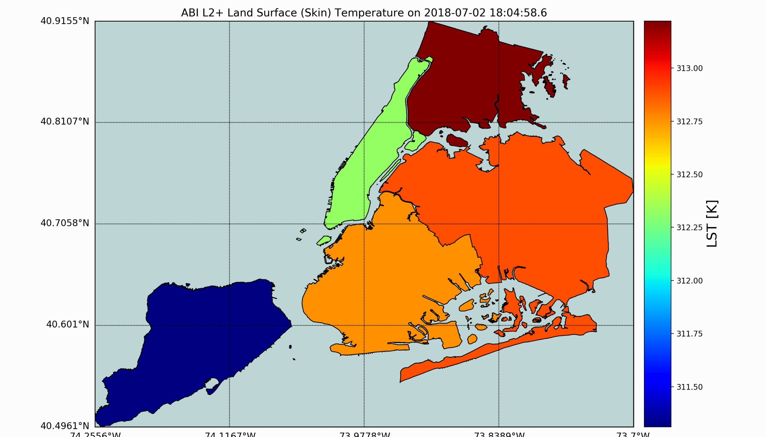
The section that clips the data finds the regions in the GOES-16 latitude/longitude points that most-closely align with the shapefile bounds. The resulting satellite image is plotted below atop the NYC shapefile:

In the figure above, we can see that around 1600 UTC time (11 a.m. NY time), there is quite a bit of warming. And upon checking the historical weather for that day, the air temperature around that time (not the same as LST) was roughly 280 K. LST is typically warmer than air temperature during the day time due to the solar heating of the surface, so we can assume the LST range of 280K-290K is fairly justified. In the next section, we will explore the average temperature of each borough by grouping each GOES-16 satellite LST pixels into its respective borough and calculating a few LST statistics for each borough.
A somewhat interesting and applicable calculation can be carried-out using the borough boundaries to approximate the mean land surface temperature (LST) for each borough of New York City. One method for determining if a data point is within a shapefile geometry is to loop through each point and use the Geospatial Data Abstraction Library (GDAL) spatial filter. This filter method is shown below:
##################
# routine that checks which points are inside each shapefile borough
##################

drv    = ogr.GetDriverByName('ESRI Shapefile') # define shapefile driver
ds_in  = drv.Open('./Borough Boundaries/geo_export_315b4419-366b-4cae-8a5a-9b945ae9112c.shp') #open shapefile
lyr_in = ds_in.GetLayer(0) # grab layer

boro_vec =  np.zeros((len(boro_unique),)) # borough vector for holding LST values
boro_count = np.zeros((len(boro_unique),)) # count points in each borough

# looping through each lat/lon point and summing LST value if it falls within one of the boroughs
for lat_pt,lon_pt,dat_pt in zip(lat_clip.flatten(),lon_clip.flatten(),dat_clip.flatten()):
    pt = ogr.Geometry(ogr.wkbPoint) # define point geometry
    pt.SetPoint_2D(0, np.float(lon_pt), np.float(lat_pt)) # set points
    lyr_in.SetSpatialFilter(pt) # filter points with shapefiles

    # loop through boroughs to find where the points lie
    for feat_in in lyr_in:
        ply = feat_in.GetGeometryRef()
        if ply.Contains(pt):
            if np.ma.isMA(dat_pt):
                continue
            boro_count[int(feat_in.GetField(0))-1]+=1
            boro_vec[int(feat_in.GetField(0))-1]+=dat_pt
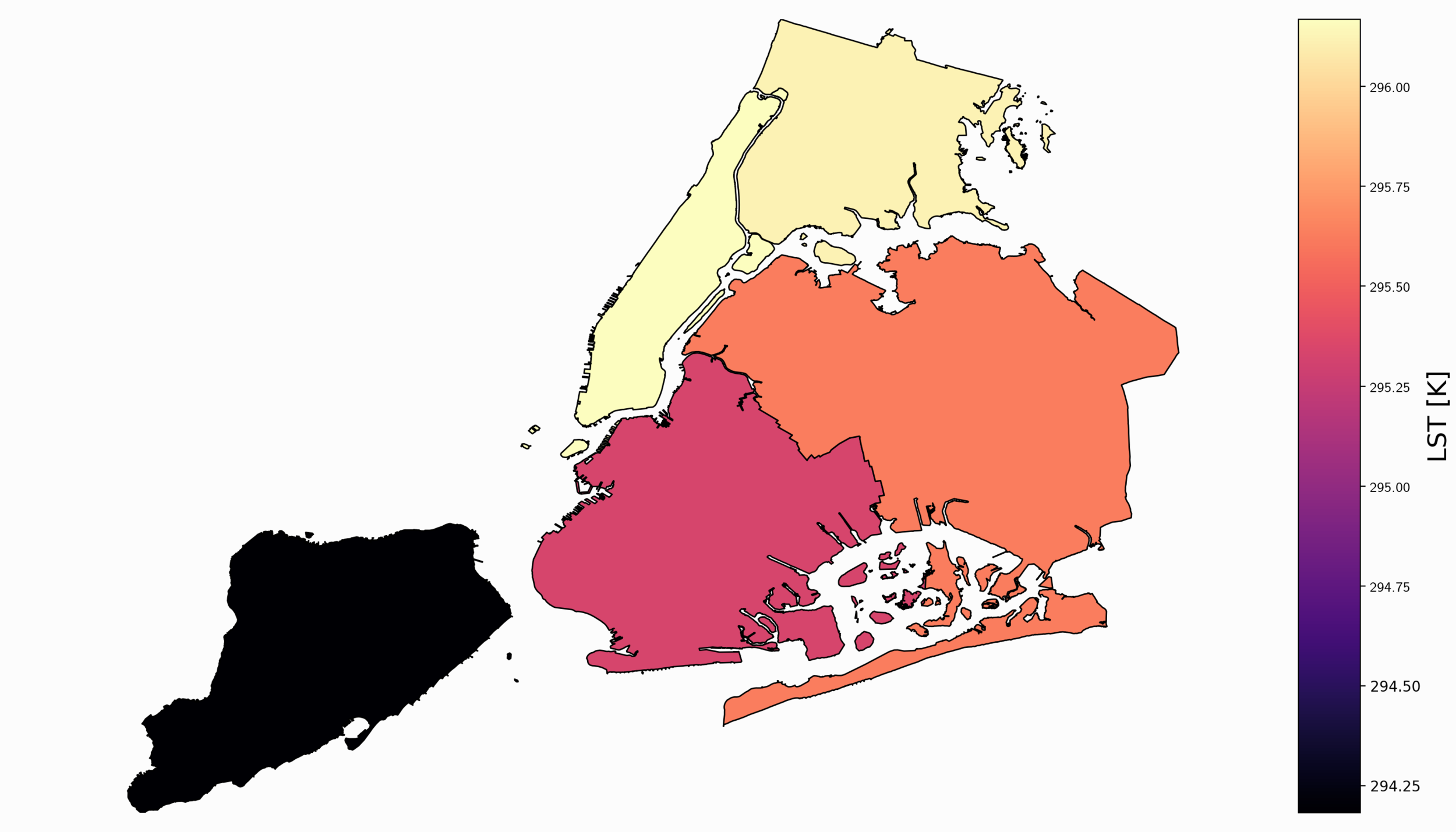
This generalized code can be added to the code in the previous section. It loops through the clipped latitude, longitude, and data file to compile statistics for each borough. Of course, this can be done for any geometry that has defined boundaries. In our case, we use the five boroughs of NYC to quantify the average LST for each borough. We can visualize the mean LST values for each borough by using a colormap that colors in each borough with a specific color that mirrors a given temperature. A plot of this is shown below:
For the given day and hour, it appears that the boroughs of the Bronx and Queens were warmer than Staten Island, Manhattan, and Brooklyn. Staten Island is the coolest borough during this peak hour. The full code to replicate this is shown below:
import matplotlib as mpl
mpl.use('TkAgg')
from mpl_toolkits.basemap import Basemap
from netCDF4 import Dataset
import os,ogr,time
import matplotlib.pyplot as plt
from matplotlib.patches import Polygon
from matplotlib.collections import PatchCollection
from matplotlib.patches import PathPatch
import numpy as np
from datetime import datetime

def lat_lon_reproj(nc_folder):
    os.chdir(nc_folder)
    full_direc = os.listdir()
    nc_files = [ii for ii in full_direc if ii.endswith('.nc')]
    g16_data_file = nc_files[0] # select .nc file
    print(nc_files[0]) # print file name

    # designate dataset
    g16nc = Dataset(g16_data_file, 'r')
    var_names = [ii for ii in g16nc.variables]
    var_name = var_names[0]

    # GOES-R projection info and retrieving relevant constants
    proj_info = g16nc.variables['goes_imager_projection']
    lon_origin = proj_info.longitude_of_projection_origin
    H = proj_info.perspective_point_height+proj_info.semi_major_axis
    r_eq = proj_info.semi_major_axis
    r_pol = proj_info.semi_minor_axis

    # grid info
    lat_rad_1d = g16nc.variables['x'][:]
    lon_rad_1d = g16nc.variables['y'][:]

    # close file when finished
    g16nc.close()
    g16nc = None

    # create meshgrid filled with radian angles
    lat_rad,lon_rad = np.meshgrid(lat_rad_1d,lon_rad_1d)

    # lat/lon calc routine from satellite radian angle vectors

    lambda_0 = (lon_origin*np.pi)/180.0

    a_var = np.power(np.sin(lat_rad),2.0) + (np.power(np.cos(lat_rad),2.0)*\
                                             (np.power(np.cos(lon_rad),2.0)+\
                                              (((r_eq*r_eq)/(r_pol*r_pol))*\
                                               np.power(np.sin(lon_rad),2.0))))
    b_var = -2.0*H*np.cos(lat_rad)*np.cos(lon_rad)
    c_var = (H**2.0)-(r_eq**2.0)

    r_s = (-1.0*b_var - np.sqrt((b_var**2)-(4.0*a_var*c_var)))/(2.0*a_var)

    s_x = r_s*np.cos(lat_rad)*np.cos(lon_rad)
    s_y = - r_s*np.sin(lat_rad)
    s_z = r_s*np.cos(lat_rad)*np.sin(lon_rad)

    # latitude and longitude projection for plotting data on traditional lat/lon maps
    lat = (180.0/np.pi)*(np.arctan(((r_eq*r_eq)/(r_pol*r_pol))*\
                                   ((s_z/np.sqrt(((H-s_x)*(H-s_x))+(s_y*s_y))))))
    lon = (lambda_0 - np.arctan(s_y/(H-s_x)))*(180.0/np.pi)

    os.chdir('../')

    return lon,lat

def data_grab(nc_folder,nc_indx):
    os.chdir(nc_folder)
    full_direc = os.listdir()
    nc_files = [ii for ii in full_direc if ii.endswith('.nc')]
    g16_data_file = nc_files[nc_indx] # select .nc file
    print(nc_files[nc_indx]) # print file name

    # designate dataset
    g16nc = Dataset(g16_data_file, 'r')
    var_names = [ii for ii in g16nc.variables]
    var_name = var_names[0]

    # data info
    data = g16nc.variables[var_name][:]
    data_units = g16nc.variables[var_name].units
    data_time_grab = ((g16nc.time_coverage_end).replace('T',' ')).replace('Z','')
    data_long_name = g16nc.variables[var_name].long_name

    # close file when finished
    g16nc.close()
    g16nc = None

    os.chdir('../')
    # print test coordinates
    print('{} N, {} W'.format(lat[318,1849],abs(lon[318,1849])))

    return data,data_units,data_time_grab,data_long_name,var_name

##################
# create dummy figure for reading shapefile and setting boundaries
##################

fig1 = plt.figure()
m1 = Basemap()
shp = m1.readshapefile('./Borough Boundaries/geo_export_315b4419-366b-4cae-8a5a-9b945ae9112c',
                       'nyc_shapefile')
plt.close(fig1) # close dummy figure
m1 = ()

##################
# plotting actual shapefile
##################

bbox = [shp[2][0],shp[2][1],shp[3][0],shp[3][1]]
fig,ax = plt.subplots(figsize=(14,8))
m = Basemap(llcrnrlon=bbox[0],llcrnrlat=bbox[1],urcrnrlon=bbox[2],
            urcrnrlat=bbox[3],resolution='i', projection='cyl')
m.readshapefile('./Borough Boundaries/geo_export_315b4419-366b-4cae-8a5a-9b945ae9112c',
                'nyc_shapefile')
m.drawmapboundary(fill_color='#bdd5d5')
parallels = np.linspace(bbox[1],bbox[3],5.) # latitudes
m.drawparallels(parallels,labels=[True,False,False,False],fontsize=12)
meridians = np.linspace(bbox[0],bbox[2],5.) # longitudes
m.drawmeridians(meridians,labels=[False,False,False,True],fontsize=12)

##################
# finding boroughs
##################

boro_array = []
for ii in m.nyc_shapefile_info:
    boro_array.append(ii['boro_code'])

boro_unique = np.unique(boro_array)


##################
# GOES-16 LST section
##################

nc_folder = './GOES_files/' # define folder where .nc files are located
lon,lat = lat_lon_reproj(nc_folder)

nc_files = [ii for ii in os.listdir(nc_folder) if ii.endswith('.nc')]
time_vec = []
for time_nc in nc_files:
    time_grab = Dataset(nc_folder+time_nc, 'r')
    time_str = ((time_grab.time_coverage_end).replace('T',' ')).replace('Z','')
    time_vec.append(datetime.strptime(time_str,'%Y-%m-%d %H:%M:%S.%f'))

nc_file_arguments = np.argsort(time_vec)

file_indx = nc_file_arguments[90] # file index selection

data,data_units,data_time_grab,data_long_name,var_name = data_grab(nc_folder,file_indx)

##################
# clipping lat/lon/data vectors to shapefile bounds
##################

llcrnr_loc_x = np.ma.argmin(np.ma.min(np.abs(np.ma.subtract(lon,bbox[0]))+\
                                      np.abs(np.ma.subtract(lat,bbox[1])),0))
llcrnr_loc = (np.ma.argmin(np.abs(np.ma.subtract(lon,bbox[0]))+\
                           np.abs(np.ma.subtract(lat,bbox[1])),0))[llcrnr_loc_x]

ulcrnr_loc_x = np.ma.argmin(np.ma.min(np.abs(np.ma.subtract(lon,bbox[0]))+\
                                      np.abs(np.ma.subtract(lat,bbox[3])),0))
ulcrnr_loc = (np.ma.argmin(np.abs(np.ma.subtract(lon,bbox[0]))+\
                           np.abs(np.ma.subtract(lat,bbox[3])),0))[ulcrnr_loc_x]

lrcrnr_loc_x = np.ma.argmin(np.ma.min(np.abs(np.ma.subtract(lon,bbox[2]))+\
                                      np.abs(np.ma.subtract(lat,bbox[1])),0))
lrcrnr_loc = (np.ma.argmin(np.abs(np.ma.subtract(lon,bbox[2]))+\
                           np.abs(np.ma.subtract(lat,bbox[1])),0))[lrcrnr_loc_x]

urcrnr_loc_x = np.ma.argmin(np.ma.min(np.abs(np.ma.subtract(lon,bbox[2]))+\
                                      np.abs(np.ma.subtract(lat,bbox[3])),0))
urcrnr_loc = (np.ma.argmin(np.abs(np.ma.subtract(lon,bbox[2]))+\
                           np.abs(np.ma.subtract(lat,bbox[3])),0))[urcrnr_loc_x]

x_bounds = [llcrnr_loc_x,ulcrnr_loc_x,lrcrnr_loc_x,urcrnr_loc_x]
y_bounds = [llcrnr_loc,ulcrnr_loc,lrcrnr_loc,urcrnr_loc]

plot_bounds = [np.min(x_bounds),np.min(y_bounds),np.max(x_bounds)+1,np.max(y_bounds)+1]

lat_clip = lat[plot_bounds[1]:plot_bounds[3],plot_bounds[0]:plot_bounds[2]]
lon_clip = lon[plot_bounds[1]:plot_bounds[3],plot_bounds[0]:plot_bounds[2]]
dat_clip = data[plot_bounds[1]:plot_bounds[3],plot_bounds[0]:plot_bounds[2]]

##################
# routine that checks which points are inside each shapefile borough
##################

drv    = ogr.GetDriverByName('ESRI Shapefile') # define shapefile driver
ds_in  = drv.Open('./Borough Boundaries/geo_export_315b4419-366b-4cae-8a5a-9b945ae9112c.shp') #open shapefile
lyr_in = ds_in.GetLayer(0) # grab layer

boro_vec =  np.zeros((len(boro_unique),)) # borough vector for holding LST values
boro_count = np.zeros((len(boro_unique),)) # count points in each borough

# looping through each lat/lon point and summing LST value if it falls within one of the boroughs
for lat_pt,lon_pt,dat_pt in zip(lat_clip.flatten(),lon_clip.flatten(),dat_clip.flatten()):
    pt = ogr.Geometry(ogr.wkbPoint) # define point geometry
    pt.SetPoint_2D(0, np.float(lon_pt), np.float(lat_pt)) # set points
    lyr_in.SetSpatialFilter(pt) # filter points with shapefiles

    # loop through boroughs to find where the points lie
    for feat_in in lyr_in:
        ply = feat_in.GetGeometryRef()
        if ply.Contains(pt):
            if np.ma.isMA(dat_pt):
                continue
            boro_count[int(feat_in.GetField(0))-1]+=1
            boro_vec[int(feat_in.GetField(0))-1]+=dat_pt

##################
# calculate each borough's mean LST and color each borough using a heat map
##################

boro_means = boro_vec/boro_count

color_bounds = [np.min(boro_means),np.max(boro_means)]
color_range = np.interp(boro_means,color_bounds,[0,255])

colors = [plt.cm.jet(int(ii)) for ii in color_range]

for boro_iter in range(0,len(boro_unique)):
    patches   = []
    for ii,jj in zip(m.nyc_shapefile_info, m.nyc_shapefile):
        if ii['boro_code']==boro_unique[boro_iter]:
            patches.append(Polygon(np.array(jj),True))

    ax.add_collection(PatchCollection(patches, facecolor= colors[boro_iter],
                                      edgecolor='k', linewidths=1., zorder=2))

img_cb = m.imshow([color_bounds],cmap='jet')
cb = m.colorbar()
data_units = ((data_units.replace('-','^{-')).replace('1','1}')).replace('2','2}')
plt.rc('text', usetex=True)
cb.set_label(r'%s $ \left[ \mathrm \right] $'% (var_name,data_units),fontsize=18)
plt.title(' on '.format(data_long_name,data_time_grab),fontsize=14)
img_cb.remove()
plt.tight_layout()
plt.savefig('nyc_borough_LST_mean.png',dpi=200,facecolor=[252/255,252/255,252/255]) # uncomment to save figure
plt.show()
I decided to investigate five days from the summer of 2018 (June 29 - July 3) during a heatwave (read about heat waves here). We can use the heatwave days to explore each borough’s daily LST profile. We do this by looping through each file, taking each borough’s averaged LST, and then stringing the multi-day profile into plot. This type of calculation is lengthy and involved, however, I have list the general process flow below to elucidate the methods used in the code:
Read the city shapefile and establish bounds
Loop through shapefile to count boroughs
Clip latitude/longitude vectors down to shapefile bounds
Loop through each file
For each file, use borough boundaries to calculate mean LST for each file (hour)
After the loop, rearrange times to plot a mean 24-hour diurnal profile during the heat wave
The resulting code and plot should be five lines that represent the mean LST trend for the heat wave for each borough of NYC.
import matplotlib as mpl
mpl.use('TkAgg')
from mpl_toolkits.basemap import Basemap
from netCDF4 import Dataset
import os,ogr,time
from datetime import datetime
import matplotlib.pyplot as plt
from matplotlib.patches import Polygon
from matplotlib.collections import PatchCollection
from matplotlib.patches import PathPatch
import numpy as np

plt.style.use('ggplot')

def lat_lon_reproj(nc_folder):
    os.chdir(nc_folder)
    full_direc = os.listdir()
    nc_files = [ii for ii in full_direc if ii.endswith('.nc')]
    g16_data_file = nc_files[0] # select .nc file
    print(nc_files[0]) # print file name

    # designate dataset
    g16nc = Dataset(g16_data_file, 'r')
    var_names = [ii for ii in g16nc.variables]
    var_name = var_names[0]

    # GOES-R projection info and retrieving relevant constants
    proj_info = g16nc.variables['goes_imager_projection']
    lon_origin = proj_info.longitude_of_projection_origin
    H = proj_info.perspective_point_height+proj_info.semi_major_axis
    r_eq = proj_info.semi_major_axis
    r_pol = proj_info.semi_minor_axis

    # grid info
    lat_rad_1d = g16nc.variables['x'][:]
    lon_rad_1d = g16nc.variables['y'][:]

    # close file when finished
    g16nc.close()
    g16nc = None

    # create meshgrid filled with radian angles
    lat_rad,lon_rad = np.meshgrid(lat_rad_1d,lon_rad_1d)

    # lat/lon calc routine from satellite radian angle vectors

    lambda_0 = (lon_origin*np.pi)/180.0

    a_var = np.power(np.sin(lat_rad),2.0) + (np.power(np.cos(lat_rad),2.0)*\
                                             (np.power(np.cos(lon_rad),2.0)+\
                                              (((r_eq*r_eq)/(r_pol*r_pol))*\
                                               np.power(np.sin(lon_rad),2.0))))
    b_var = -2.0*H*np.cos(lat_rad)*np.cos(lon_rad)
    c_var = (H**2.0)-(r_eq**2.0)

    r_s = (-1.0*b_var - np.sqrt((b_var**2)-(4.0*a_var*c_var)))/(2.0*a_var)

    s_x = r_s*np.cos(lat_rad)*np.cos(lon_rad)
    s_y = - r_s*np.sin(lat_rad)
    s_z = r_s*np.cos(lat_rad)*np.sin(lon_rad)

    # latitude and longitude projection for plotting data on traditional lat/lon maps
    lat = (180.0/np.pi)*(np.arctan(((r_eq*r_eq)/(r_pol*r_pol))*\
                                   ((s_z/np.sqrt(((H-s_x)*(H-s_x))+(s_y*s_y))))))
    lon = (lambda_0 - np.arctan(s_y/(H-s_x)))*(180.0/np.pi)

    os.chdir('../')

    return lon,lat

def data_grab(nc_folder,nc_indx):
    os.chdir(nc_folder)
    full_direc = os.listdir()
    nc_files = [ii for ii in full_direc if ii.endswith('.nc')]
    g16_data_file = nc_files[nc_indx] # select .nc file
    print(nc_files[nc_indx]) # print file name

    # designate dataset
    g16nc = Dataset(g16_data_file, 'r')
    var_names = [ii for ii in g16nc.variables]
    var_name = var_names[0]

    # data info
    data = g16nc.variables[var_name][:]
    data_units = g16nc.variables[var_name].units
    data_time_grab = ((g16nc.time_coverage_end).replace('T',' ')).replace('Z','')
    data_long_name = g16nc.variables[var_name].long_name

    # close file when finished
    g16nc.close()
    g16nc = None

    os.chdir('../')
    # print test coordinates
    print('{} N, {} W'.format(lat[318,1849],abs(lon[318,1849])))

    return data,data_units,data_time_grab,data_long_name,var_name

##################
# reading shapefile and setting boundaries
##################

drv    = ogr.GetDriverByName('ESRI Shapefile') # define shapefile driver
ds_in  = drv.Open('./Borough Boundaries/geo_export_315b4419-366b-4cae-8a5a-9b945ae9112c.shp') #open shapefile
lyr_in = ds_in.GetLayer(0) # grab layer
shp = lyr_in.GetExtent()

bbox = [shp[0],shp[2],shp[1],shp[3]]

##################
# finding boroughs
##################

boro_array = []
for ii in range(0,(lyr_in.GetFeatureCount())):
    boro_array.append((lyr_in.GetFeature(ii)).GetField(0))

boro_unique = np.unique(boro_array)
boro_str = ['']*len(boro_unique)

##################
# clipping lat/lon/data vectors to shapefile bounds
##################

nc_folder = './GOES_files/' # define folder where .nc files are located
lon,lat = lat_lon_reproj(nc_folder)

llcrnr_loc_x = np.ma.argmin(np.ma.min(np.abs(np.ma.subtract(lon,bbox[0]))+\
                                      np.abs(np.ma.subtract(lat,bbox[1])),0))
llcrnr_loc = (np.ma.argmin(np.abs(np.ma.subtract(lon,bbox[0]))+\
                           np.abs(np.ma.subtract(lat,bbox[1])),0))[llcrnr_loc_x]

ulcrnr_loc_x = np.ma.argmin(np.ma.min(np.abs(np.ma.subtract(lon,bbox[0]))+\
                                      np.abs(np.ma.subtract(lat,bbox[3])),0))
ulcrnr_loc = (np.ma.argmin(np.abs(np.ma.subtract(lon,bbox[0]))+\
                           np.abs(np.ma.subtract(lat,bbox[3])),0))[ulcrnr_loc_x]

lrcrnr_loc_x = np.ma.argmin(np.ma.min(np.abs(np.ma.subtract(lon,bbox[2]))+\
                                      np.abs(np.ma.subtract(lat,bbox[1])),0))
lrcrnr_loc = (np.ma.argmin(np.abs(np.ma.subtract(lon,bbox[2]))+\
                           np.abs(np.ma.subtract(lat,bbox[1])),0))[lrcrnr_loc_x]

urcrnr_loc_x = np.ma.argmin(np.ma.min(np.abs(np.ma.subtract(lon,bbox[2]))+\
                                      np.abs(np.ma.subtract(lat,bbox[3])),0))
urcrnr_loc = (np.ma.argmin(np.abs(np.ma.subtract(lon,bbox[2]))+\
                           np.abs(np.ma.subtract(lat,bbox[3])),0))[urcrnr_loc_x]

x_bounds = [llcrnr_loc_x,ulcrnr_loc_x,lrcrnr_loc_x,urcrnr_loc_x]
y_bounds = [llcrnr_loc,ulcrnr_loc,lrcrnr_loc,urcrnr_loc]

plot_bounds = [np.min(x_bounds),np.min(y_bounds),np.max(x_bounds)+1,np.max(y_bounds)+1]

lat_clip = lat[plot_bounds[1]:plot_bounds[3],plot_bounds[0]:plot_bounds[2]]
lon_clip = lon[plot_bounds[1]:plot_bounds[3],plot_bounds[0]:plot_bounds[2]]

##################
# GOES-16 LST section
##################

time_hour_vec,data_hour_vec,total_time_vec = [],[],[]

nc_files = [ii for ii in os.listdir(nc_folder) if ii.endswith('.nc')]
for file_indx in range(0,len(nc_files)):

    data,data_units,data_time_grab,data_long_name,var_name = data_grab(nc_folder,file_indx)

    dat_clip = data[plot_bounds[1]:plot_bounds[3],plot_bounds[0]:plot_bounds[2]]

    ##################
    # routine that checks which points are inside each shapefile borough
    ##################

    boro_vec =  np.zeros((len(boro_unique),)) # borough vector for holding LST values
    boro_count = np.zeros((len(boro_unique),)) # count points in each borough

    # looping through each lat/lon point and summing LST value if it falls within one of the boroughs

    for lat_pt,lon_pt,dat_pt in zip(lat_clip.flatten(),lon_clip.flatten(),dat_clip.flatten()):
        pt = ogr.Geometry(ogr.wkbPoint) # define point geometry
        pt.SetPoint_2D(0, np.float(lon_pt), np.float(lat_pt)) # set points
        lyr_in.SetSpatialFilter(pt) # filter points with shapefiles

        # loop through boroughs to find where the points lie
        for feat_in in lyr_in:
            ply = feat_in.GetGeometryRef()
            if ply.Contains(pt):
                if np.ma.isMA(dat_pt):
                    continue
                if boro_str[int(feat_in.GetField(0))-1]=='':
                    boro_str[int(feat_in.GetField(0))-1] = feat_in.GetField(1)
                boro_count[int(feat_in.GetField(0))-1]+=1
                boro_vec[int(feat_in.GetField(0))-1]+=dat_pt

    ##################
    # Adding hour of day and mean LST to vectors for later analysis
    ##################

    t1 = datetime.strptime(data_time_grab,'%Y-%m-%d %H:%M:%S.%f')

    boro_means = boro_vec/boro_count
    total_time_vec.append(t1)
    time_hour_vec.append(t1.hour)
    data_hour_vec.append(boro_means)

time_hour_vec = np.array(time_hour_vec)
data_hour_vec = np.array(data_hour_vec)

##################
# Plotting diurnal LST profile for each borough
##################
daily_mean = []
fig,ax = plt.subplots(figsize=(14,9))
for jj in range(0,np.shape(data_hour_vec)[1]):
    plot_var = []
    curr_vars = np.array([data_hour_vec[ii][jj] for ii in range(0,np.shape(data_hour_vec)[0])])
    for hour in np.unique(time_hour_vec):
        plot_var.append(np.nanmean(curr_vars[np.where(time_hour_vec==hour)]))

    ax.plot(np.unique(time_hour_vec),plot_var,marker='o',linestyle='-',
            markersize=8,linewidth=3,markeredgecolor='k',
            label=boro_str[jj])
    daily_mean.append(np.nanmean(plot_var))

ax.set_xlabel('Hour of Day',fontsize=18)
ax.set_ylabel('LST [K]',fontsize=18)
ax.tick_params(axis='both',which='major',labelsize=14)
ax.legend(fontsize=16)
data_units = ((data_units.replace('-','^{-')).replace('1','1}')).replace('2','2}')
ax.set_title(' from  - '.format(\
    data_long_name,
    datetime.strftime(np.min(total_time_vec),'%b %d, %Y'),
    datetime.strftime(np.max(total_time_vec),'%b %d, %Y')),
             fontsize=18)
plt.tight_layout()
plt.savefig('nyc_borough_diurnal_plot.png',dpi=200,
            facecolor=[252/255,252/255,252/255]) # uncomment to save figure
plt.show()

From the heat wave data taken from June 29th - July 3rd, we see the general daily trend in land surface temperature. If we translate the data from UTC to local time, we can conclude that peak heating occurs between 12 p.m. - 3 p.m. If we take the mean of each diurnal profile, we can quantitatively cite the mean daily temperature for each borough during the heat wave:
Manhattan : 302.2 K
Bronx : 302.2 K
Brooklyn : 301.7 K
Queens : 301.6 K
Staten Island : 301.6 K
We can conclude that the mean temperatures for each borough are about the same during the heat wave, though we can observe certain behaviors for each borough. Manhattan appears to hold on to heat more than the other boroughs, and Staten Island appears to be the coolest at any given time. I imagine the particularities of each borough would emerge if more data was added to the analysis.
Furthermore, if we focus on one borough, we can observe the temperature’s standard deviation for each hour during the heat wave. This will give us an idea of the span of the mean temperature for each hour. The plot is shown below for Manhattan:

This concludes the second entry into the Python satellite imagery analysis tutorial series. In the first entry, I explored netCDF files and Python’s Basemap toolkit for reading and plotting geographic data and satellite imagery. In this tutorial, I introduced shapefiles as tools for clipping satellite data to city boundaries. I also demonstrated some powerful Python techniques for calculating mean parameters of particular geographic regions, using shapefiles and LST data. We were able to investigate the mean LST during a heat wave for New York City, while also visualizing the standard deviation of the diurnal LST profile. In the upcoming entry, I will use the National Land Cover Database (NLCD) and digital elevation maps to understand the distribution of LST under varying surface parameters.
See More in Python and GIS: