Google Trends x Yahoo Finance Analysis in Python
Python has a multitude of libraries dedicated to scraping the internet in various ways. For example, Google Trends is a product produced by Google that analyzes search history and publishes the popularity of search terms over time. One user created an algorithm to pull trend data from Google using Python in a package called pytrends. Another such library uses Python to pull stock information from Yahoo Stocks in a package called yfinance. Both of these libraries will be used to plot and compare finance and trend data over time using Python scripts. The methods outlined in this tutorial could be applied to areas in finance, data analytics, and data visualization in general.
user:~ $sudo pip3 install pytrends finance
If the packages were installed correctly, we can head to Python 3.x and attempt to import the packages in order to verify their functionality and that everything installed correctly. Below I have included a test script that should test the import and basic function of both packages:
from pytrends import dailydata
import yfinance as fin
from datetime import datetime

# selecting ticker for yahoo finance
ticker = 'INTC' # which stock to search for
ticker_handle = fin.Ticker(ticker) # ticker handler
company_name = ticker_handle.info.get('shortName')

# getting 30 days of trend and finance data
t_now = datetime.now()
t_prev= datetime.fromtimestamp(t_now.timestamp()-(3600*24*30))
trends = dailydata.get_daily_data(company_name,t_prev.year,t_prev.month,
                                  t_now.year,t_now.month)
fin_data = fin.download(ticker,start=t_prev.strftime('%Y-%m-%d'),
                        end=t_now.strftime('%Y-%m-%d'))

print('Most Recent Stock Price for  on : $'.format(\
    company_name,fin_data.index[-1].strftime('%m-%d-%Y'),fin_data.values[-1,3]))
print('Most Recent Google Trend Data for  on : '.format(company_name,
                                                       trends.index[-1].strftime('%m-%d-%Y'),
                                                                      trends.values[-1,3]))
The example above should print out the following, with adjusted times based on the run date:
Intel Corporation:2019-12-01 2019-12-31
Intel Corporation:2020-01-01 2020-01-31

[*********************100%***********************]  1 of 1 completed
Most Recent Stock Price for Intel Corporation on 01-17-2020: $59.60
Most Recent Google Trend Data for Intel Corporation on 01-17-2020: 0.60
The code above grabs the available Google Trends data from the last 30 days (likely, 2 months of trend data), and then grabs 30 days worth of finance data from Yahoo Finance, and prints out the last value from each database. In the case above, ‘INTC’ is used as the input to the Yahoo Finance database, and we then tell Google Trends to return the trend data for ‘Intel Corporation.’ The resulting data is the stock closing price on the 17th of January, 2020; a value of $59.60. The resulting trend data is 0.6, indicating a medium-level popularity in search data with Google for the Intel Corporation (the value printed is the scaled data, ranging from 0-1, where 1 indicates a highly popular period, and 0 indicates a highly unpopular time period).
Now that the stock and trend packages are downloaded and have been tested, we can begin to look at how the two behave over time by plotting them together. The code below grabs data from the AAPL (Apple) stock and compares it with the “Apple, Inc.” Google Trends search for the months of September - December 2019:
from pytrends import dailydata
import numpy as np
import matplotlib.pyplot as plt
import yfinance as fin
import datetime

#
######################################
# INPUTS
######################################
#
ticker = 'AAPL' # which stock to search for
date_range = [9,1,2019,12,30,2019] # date range of interest, format: 'month,day,year'
fin_indx = 0 #Prices: 0=Open,1=High,2=Low,3=Close,4=Adj Close,5=Volume
trend_indx = 3 #Popularity: 0=unscaled 0-100, 1=monthly, 2=isPartial, 3=scaled

#
######################################
# DATE AND DATA HANDLING
######################################
#
start_t = datetime.datetime(date_range[2],date_range[0],date_range[1])
end_t   = datetime.datetime(date_range[5],date_range[3],date_range[4])

ticker_handle = fin.Ticker(ticker)
trends = dailydata.get_daily_data(ticker_handle.info.get('shortName').split(' ')[0],
                                  date_range[2],date_range[0],
                                  date_range[5],date_range[3])

fin_data = fin.download(ticker,start=start_t.strftime('%Y-%m-%d'),
                        end=end_t.strftime('%Y-%m-%d'))

#
######################################
# PLOTTING ROUTINES
######################################
#
plt.style.use('ggplot')
fig,ax = plt.subplots(figsize=(14,9))

fin_keys = fin_data.keys() # keys for naming plotted finance data
trend_keys = trends.keys() # keys for naming plotted trends data

fin_x   = [ii.timestamp() for ii in fin_data.index] # formatting dates into timestamp for plotting
fin_y   = (fin_data.values)[:,fin_indx] # trend data to plot

trend_x = [ii.timestamp() for ii in trends.index] # formatting dates into timestamp for plotting
trend_y = (trends.values)[:,trend_indx] # trend data to plot

trend_start_indx = np.argmin(np.abs(np.subtract(trend_x,fin_x[0])))
trend_end_indx   = np.argmin(np.abs(np.subtract(trend_x,fin_x[-1])))
trend_x = trend_x[trend_start_indx:trend_end_indx+1] # align trends + stock $
trend_y = trend_y[trend_start_indx:trend_end_indx+1] # align trends + stock $

scat1 = ax.scatter(trend_x,trend_y,color=plt.cm.tab20(0),s=120) # scatter trend data

ax.set_ylabel('Trend: '+(trend_keys[trend_indx].replace('_',' ')),
              fontsize=20,color=plt.cm.tab20(0))
x_ticks = ax.get_xticks()
x_str_labels = [(datetime.datetime.fromtimestamp(ii)).strftime('%m-%d-%Y') for ii in x_ticks]
ax.set_xticklabels(x_str_labels) # format dates on x-axis
ax.set_xlabel('Time [Month-Day-Year]',fontsize=20)

ax2 = ax.twinx() # twin axis to plot both data on the same plot
ax2.grid(False) # this prevents the axes from being too messy
scat2 = ax2.scatter(fin_x,fin_y,color=plt.cm.tab20(2),s=120) # scatter finance data
ax2.set_ylabel(fin_keys[fin_indx]+' Price [$ USD]',fontsize=20,color=plt.cm.tab20(2))

plt.title(ticker+' ({}) '.format(ticker_handle.info.get('shortName'))+' from {} - {}'.format(start_t.strftime('%m/%d/%Y'),
                                        end_t.strftime('%m/%d/%Y')),
          fontsize=20)

plt.show() # show plot
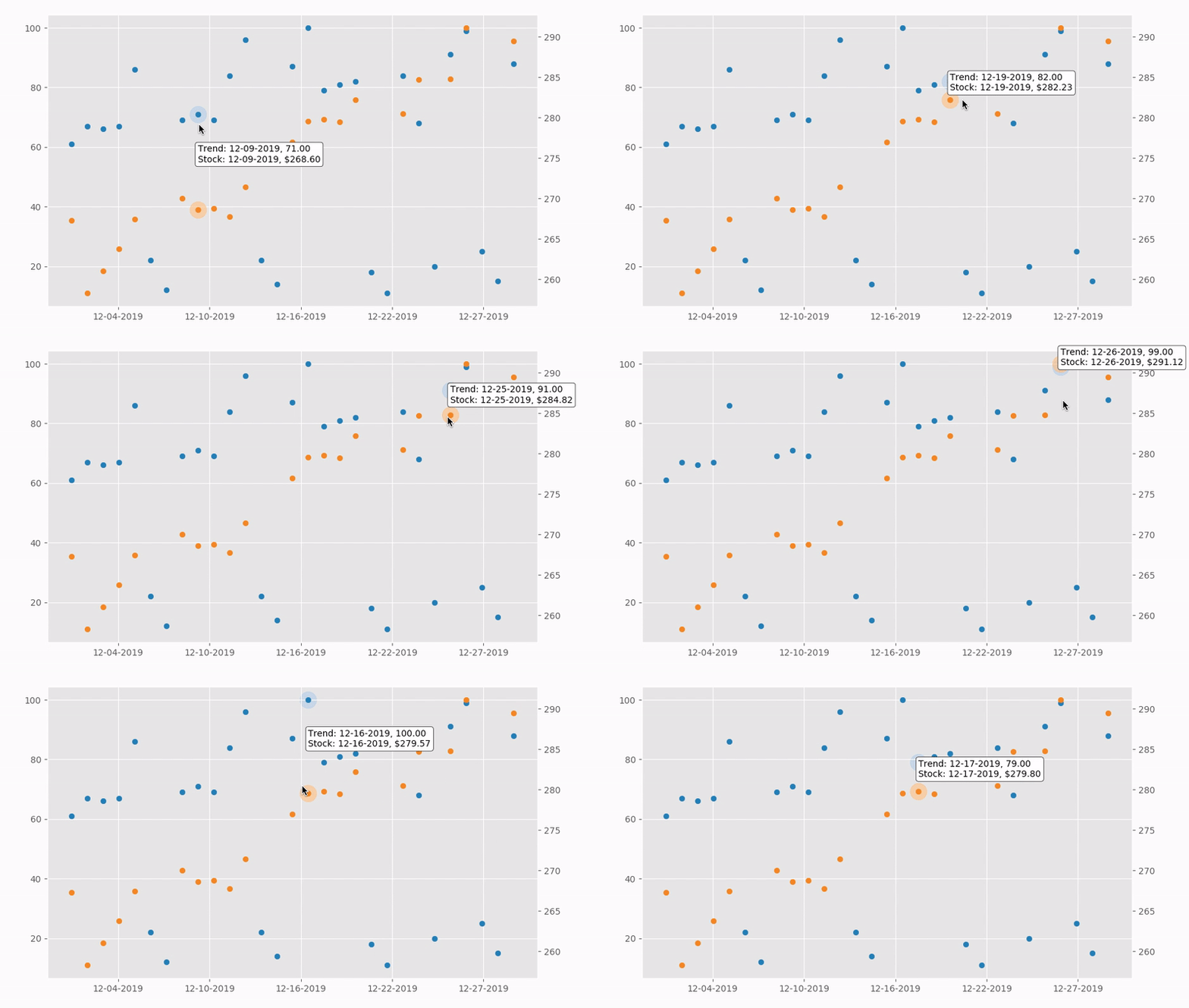
The resulting plot is shown below:
We can see just how the trends and stock prices are correlated and how specific events can be seen on both the trends and stock price changes. For example, on September 9, 2019 Apple was trending at its peak over the three month period, and this can be correlated to the announcement of the iPhone 11. Two other peaks over the three month period can be attributed to Black Friday sales and Christmas sales. The subtler changes in stock price can be correlated to performance of the Apple brand.
One statistical measure for comparing two different data is called correlation. Correlation involves the covariance between two variables and their two standard deviations. The correlation coefficient can be written as:
where rx,y is the correlation coefficient, x is the first variable, y is the second variable, k is the index of each sample, and N is the total number of samples in a given set of data. An overline, in the case of x, defines the mean of the given variable x.
In the code and plot below, I introduce the correlation between trend and stock opening price for AAPL (Apple Inc.) for all of 2019:
from pytrends import dailydata
import numpy as np
import matplotlib.pyplot as plt
import yfinance as fin
import datetime

#
######################################
# INPUTS
######################################
#
ticker = 'AAPL' # which stock to search for
date_range = [1,1,2019,12,30,2019] # date range of interest, format: 'month,day,year'
fin_indx = 0 #Prices: 0=Open,1=High,2=Low,3=Close,4=Adj Close,5=Volume
trend_indx = 3 #Popularity: 0=unscaled 0-100, 1=monthly, 2=isPartial, 3=scaled

#
######################################
# DATE AND DATA HANDLING
######################################
#
start_t = datetime.datetime(date_range[2],date_range[0],date_range[1])
end_t   = datetime.datetime(date_range[5],date_range[3],date_range[4])

ticker_handle = fin.Ticker(ticker)
trends = dailydata.get_daily_data(ticker_handle.info.get('shortName').split(' ')[0],
                                  date_range[2],date_range[0],
                                  date_range[5],date_range[3])

fin_data = fin.download(ticker,start=start_t.strftime('%Y-%m-%d'),
                        end=end_t.strftime('%Y-%m-%d'))

#
######################################
# Time aligning routines
######################################
#
fin_keys = fin_data.keys() # keys for naming plotted finance data
trend_keys = trends.keys() # keys for naming plotted trends data

fin_x   = [ii.timestamp() for ii in fin_data.index] # formatting dates into timestamp for plotting
fin_y   = (fin_data.values)[:,fin_indx] # trend data to plot

trend_x = [ii.timestamp() for ii in trends.index] # formatting dates into timestamp for plotting
trend_y = (trends.values)[:,trend_indx] # trend data to plot

trend_start_indx = np.argmin(np.abs(np.subtract(trend_x,fin_x[0])))
trend_end_indx   = np.argmin(np.abs(np.subtract(trend_x,fin_x[-1])))
trend_y = [trend_y[np.argmin(np.abs(np.subtract(ii,trend_x)))] for ii in fin_x] # align trends + stock $
trend_x = [trend_x[np.argmin(np.abs(np.subtract(ii,trend_x)))] for ii in fin_x] # align trends + stock $
#
#######################################
# correlation calculation
#######################################
#
corr_xy_array = [0.0]
for ii in range(1,len(fin_y)):
    mean_x = np.nanmean(trend_y[0:ii])
    mean_y = np.nanmean(fin_y[0:ii])
    sigma_x = np.sqrt(np.nansum(np.power(trend_y[0:ii]-mean_x,2.0)))
    sigma_y = np.sqrt(np.nansum(np.power(fin_y[0:ii]-mean_y,2.0)))
    corr_xy = (np.nansum(np.multiply((np.subtract(trend_y[0:ii],mean_x)),
                                     np.subtract(fin_y[0:ii],mean_y))))\
              /(sigma_x*sigma_y)
    if np.isnan(corr_xy):
        corr_xy = 0.0
    corr_xy_array.append(corr_xy)

#
#######################################
# PLOTTING
#######################################
#
plt.style.use('ggplot')
fig,axs = plt.subplots(2,1,figsize=(14,9),sharex=True)

ax = axs[0]
ax.scatter(trend_x,trend_y,color=plt.cm.tab20(0))
ax2 = ax.twinx()
ax2.grid(False)
ax2.scatter(fin_x,fin_y,color=plt.cm.tab20(2))

ax.set_ylabel('Trend: '+(trend_keys[trend_indx].replace('_',' ')),color=plt.cm.tab20(0),fontsize=20)
ax2.set_ylabel(fin_keys[fin_indx]+' Price [$ USD]',color=plt.cm.tab20(2),fontsize=20)

ax3 = axs[1]
scat3 = ax3.scatter(fin_x,corr_xy_array,color=plt.cm.tab20(4)) # scatter trend data
ax3.set_ylabel('Correlation',
              fontsize=20,color=plt.cm.tab20(4))
x_ticks = ax3.get_xticks()
x_str_labels = [(datetime.datetime.fromtimestamp(ii)).strftime('%m-%d-%Y') for ii in x_ticks]
ax3.set_xticklabels(x_str_labels) # format dates on x-axis
ax3.set_xlabel('Time [Month-Day-Year]',fontsize=20)
ax2.set_xticklabels(x_str_labels)

ax.set_title(ticker+' ({}) '.format(ticker_handle.info.get('shortName'))+' from {} - {}'.format(start_t.strftime('%m/%d/%Y'),
                                        end_t.strftime('%m/%d/%Y')),
          fontsize=20)

plt.show() # show plot
We can see that the correlation function follows a lot of the momentum of either positive or negative trends in stock price. We can see that for roughly 3/4 of the year there is a negative correlation between stock price and trend. This indicates that the absence of search related to Apple was correlated to an increase in stock price. And the last quarter of 2019 indicates that there was a positive correlation between increase in stock price and search popularity; meaning that there was a direct correlation between search and increase in stock price. This change in the last quarter can be attributed to some of the sales related to the iPhone 11 as well as other products.
This short introduction to Google Trends and Yahoo Finance in Python is meant as a starting point for those interested in analyzing data related to stocks and peripheral company information. Other sources of information related to company stocks can also be used to correlate stock price, such as news, weather, and even company earnings and expenditures. Python is a powerful tool that can be used to mine and analyze publicly available data. Libraries and module help maintain Python as one of the most important programming languages of the 21st century. Traditional statistical tools are also helpful for understanding relationships between stocks and peripheral data - and in this tutorial I merely covered one: correlation. The time series correlation can give us some insight into how search trends relate to company stock price, and can perhaps be used as a tool for predicting the behavior of company stock prices.
See More in Python and Data Analysis:


