Audio Processing in Python Part III: Guitar String Theory and Frequency Analysis
There are many advantages to knowing the real-time spectrum of a signal. One such example is in music. Guitar tuners use live spectrograms to tell the musician whether their instrument is tuned at the correct frequencies. In this continuation of the audio processing in Python series I will be discussing the live frequency spectrum and its application to tuning a guitar. I will introduce the idea of nodes and antinodes of a stringed instrument and the physical phenomena known as harmonics. This will give us a better idea of how to tune the guitar string-by-string and also discern the notes of a given chord - all calculated using the FFT function in Python.

Fundamentals and Harmonics of a Vibrating String
When a string is plucked it is capable of emitting a range of frequencies based on its length and material properties. We can use the wave equation in one dimension to represent the behavior of a string under excitation:
where t is time, x is along the length of the string, u is the amplitude deflection of the string, and c is the speed of the wave along the string.
The T in the wave speed is an approximate tension, and μ is the mass per unit length of the string. And if we assume a solution of sinusoidal profile:
Upon plugging this solution back into the wave equation, we can find that the speed of the wave is related to the wave number and frequency by:
For a guitar, we can assume both ends of the string are fixed:

Figure 1: Fixed string that represents a stringed instrument. We will be suing this geometry to calculate modes of a vibrating string.
Using the wave solution above, we can simplify the unknowns in the equation by taking advantage of the properties of the string:
We can simplify a bit using rules of exponentials:
And introducing the cosines and sines using Euler’s relation:
Simplifying:
Taking only the real (physical) part:
where C has absorbed the other constants, k is the wavenumber, and ω is the angular frequency. From here we can impose another boundary condition on the right side of the string at x = l:
We can now use the relationship that we found earlier relating the wave speed to the frequency and wave number:
Which gives us the true definition of the standing wave frequency modes:
This states that with knowledge of the speed of the wave in the material and the length of the string, we can compute and predict the fundamental and harmonic modes of the system. Things get a little trickier, however, when discussing the speed of the wave. In order to predict the speed of the wave, we need to return to the definition of the speed of the wave, shown above:
Therefore, in the case of tuning a guitar, since we know roughly the length of the string, the mass per unit length of the string, and the target frequency (set by musical standards), we can predict the needed tension. A guitar also has the same length of string for each of its six strings, which means that the mass per unit length or tension need to change in order for the frequency to change. This is why we see different types of strings on a guitar.

Figure 2: The fundamental mode of a standing wave on a string. Using the equation derived above, we can calculate the fundamental modes of a guitar using the length of the string, the density of the string, and information about the tension on the string.
The fundamental mode is shown above. The fundamental is the lowest natural mode of vibration of the system. In the case of a guitar, we expect this frequency to be the open note of any of the six strings. The notes above the fundamental are called harmonics, and they can be calculated by increase the values of n in the equation above for frequency. Below I have plotted the first and second harmonics (second and third notes on the string).

Figure 3: First harmonic of the string (second note).

Figure 4: Second harmonic of the string (third note).
Harmonics are integer multiples (in most systems), so to find the harmonics in a recording, we can look at the fundamental and calculate if there are integer multiples of that note higher in the frequency spectrum. Now that we understand modes of a string a bit more, we can look at the strings on a guitar.

The USB microphone is perfect for audio projects that involve Raspberry Pi due to its slim profile, long attached USB cable, and its frequency response. This USB microphone can be used for acoustic signal processing, voice recognition, musical instrument recording, or engineering applications in machine noise monitoring.
Included in package:
USB Condenser Microphone
USB Microphone Specs:
1.5 m long cable
Omnidirectional response pattern
USB 2.0 (works with Raspberry Pi)
50 Hz - 16 kHz frequency response
Microphone Size (without windscreen): 6.5 cm x 0.7 cm
44.1 kHz/48kHz USB Sample Rate Selection
-38 dB ± 3 dB Sensitivity
Acoustic Breakdown of The Guitar
The guitar is a six-stringed instrument with the following frequency distribution (Wikipedia):
| Guitar Frequencies [Hz] | |
|---|---|
| E | 329.63 |
| B | 246.94 |
| G | 196.00 |
| D | 146.83 |
| A | 110.00 |
| E | 82.41 |
The frequencies above are for the standard tuning method of playing guitar. The lowest string on the guitar oscillates at about 82 Hz, and the highest string on the guitar oscillates at about 330 Hz. This means that when we take the Fast Fourier Transform of the guitar, we expect to see six large peaks when the guitar is strummed without any fingering. We may also see harmonics and other peaks depending on the shape and geometry of the guitar as well, though the shape of the body is a whole discuss itself and I will not in-depth about that type of behavior. We will assume all the dominant peaks will be fundamentals or harmonics, and will ignore the others.
Video showing higher-order modes of a close-up A-String on a guitar.
When we press down a guitar string, we are effectively changing the length of the string, which results in a higher frequency (see frequency equation above). If we press a string down halfway between each endpoint, we can expect a frequency that is twice the fundamental. Using the change in string length and the frequency equation above, we can calculate every note on a guitar or any standing wave stringed instrument. From here, we can investigate and test the frequency content in a guitar by using the FFT function in Python.
Measuring the Frequency Content of a Guitar

In this section I will be using fairly advanced Python programming to do the following:
Record 1 second of audio data using a USB mic [tutorial here]
Subtract background noise in time and spectral domain
Calculate FFT for guitar strum [tutorial here]
Plot frequency spectra of guitar strum
Annotate 6 peak frequencies related using a peak finding algorithm
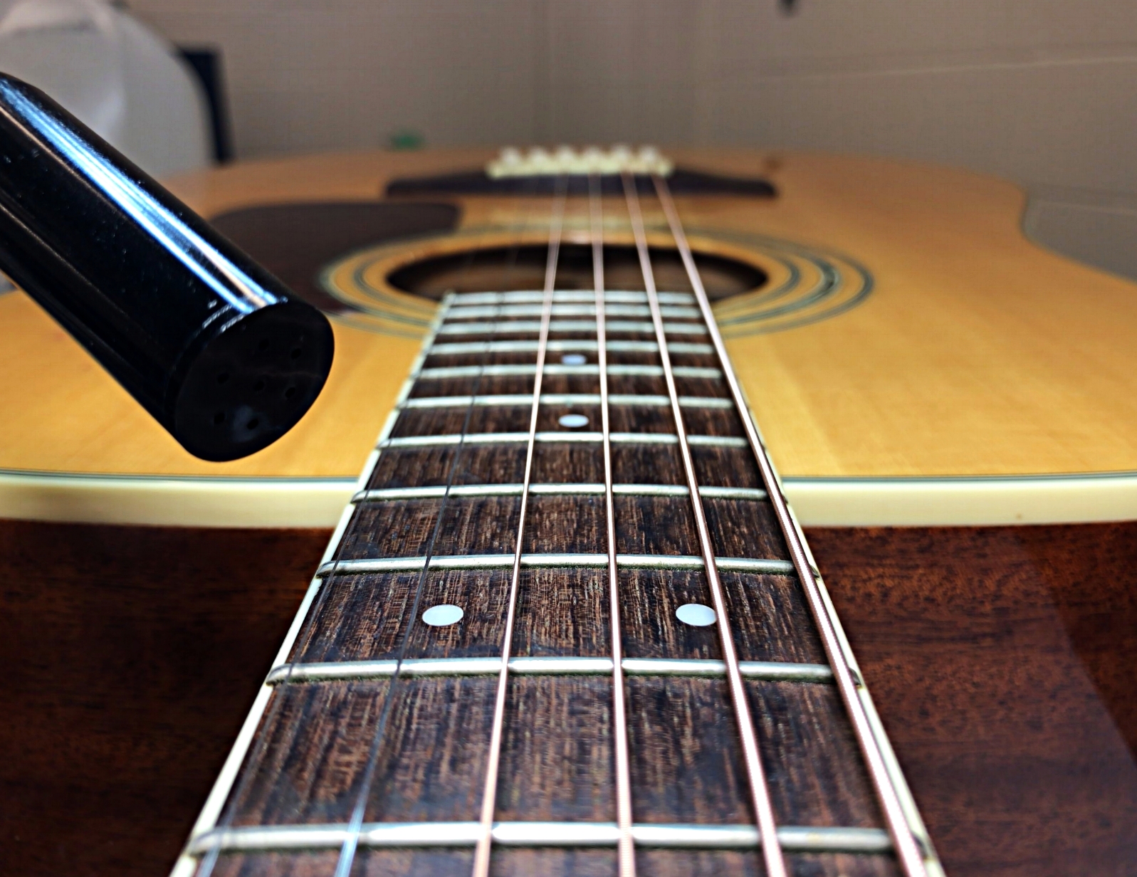
I am using an acoustic guitar from Fender to produce the modes and as the stringed instrument for investigation. The guitar is tuned to a near-standard tuning configuration. The code for the algorithm outlined above is shown below:
import pyaudio
import matplotlib.pyplot as plt
import numpy as np
import time

plt.style.use('ggplot')

form_1 = pyaudio.paInt16 # 16-bit resolution
chans = 1 # 1 channel
samp_rate = 44100 # 44.1kHz sampling rate
chunk = 44100 # samples for buffer (more samples = better freq resolution)
dev_index = 2 # device index found by p.get_device_info_by_index(ii)

audio = pyaudio.PyAudio() # create pyaudio instantiation

# mic sensitivity correction and bit conversion
mic_sens_dBV = -47.0 # mic sensitivity in dBV + any gain
mic_sens_corr = np.power(10.0,mic_sens_dBV/20.0) # calculate mic sensitivity conversion factor

# compute FFT parameters
f_vec = samp_rate*np.arange(chunk/2)/chunk # frequency vector based on window size and sample rate
mic_low_freq = 70 # low frequency response of the mic (mine in this case is 100 Hz)
low_freq_loc = np.argmin(np.abs(f_vec-mic_low_freq))

# prepare plot for live updating
plt.ion()
fig = plt.figure(figsize=(12,5))
ax = fig.add_subplot(111)
annot = ax.text(np.exp(np.log((0.8*f_vec[-1]))/2),0,"Measuring Noise...",\
                fontsize=30,horizontalalignment='center')
y = np.zeros((int(np.floor(chunk/2)),1))
line1, = ax.plot(f_vec,y)
plt.xlabel('Frequency [Hz]',fontsize=22)
plt.ylabel('Amplitude [Pa]',fontsize=22)
plt.grid(True)
plt.annotate(r'$\Delta f_{max}$: %2.1f Hz' % (samp_rate/(2*chunk)),xy=(0.7,0.9),xycoords='figure fraction',fontsize=16)
ax.set_xscale('log')
ax.set_xlim([1,0.8*samp_rate])
plt.pause(0.0001)

# create pyaudio stream
stream = audio.open(format = form_1,rate = samp_rate,channels = chans, \
                    input_device_index = dev_index,input = True, \
                    frames_per_buffer=chunk)

# some peak-finding and noise preallocations
peak_shift = 5
noise_fft_vec,noise_amp_vec = [],[]
annot_array,annot_locs = [],[]
annot_array.append(annot)
peak_data = []
noise_len = 5
ii = 0

# loop through stream and look for dominant peaks while also subtracting noise
while True:

    # read stream and convert data from bits to Pascals
    stream.start_stream()
    data = np.fromstring(stream.read(chunk),dtype=np.int16)
    if ii==noise_len:
        data = data-noise_amp
    data = ((data/np.power(2.0,15))*5.25)*(mic_sens_corr)
    stream.stop_stream()

    # compute FFT
    fft_data = (np.abs(np.fft.fft(data))[0:int(np.floor(chunk/2))])/chunk
    fft_data[1:] = 2*fft_data[1:]

    # calculate and subtract average spectral noise
    if ii<noise_len:
        if ii==0:
            print("Stay Quiet, Measuring Noise...")
        noise_fft_vec.append(fft_data)
        noise_amp_vec.extend(data)
        print(".")
        if ii==noise_len-1:
            noise_fft = np.max(noise_fft_vec,axis=0)
            noise_amp = np.mean(noise_amp_vec)
            print("Now Recording")
        ii+=1
        continue

    fft_data = np.subtract(fft_data,noise_fft) # subtract average spectral noise

    # plot the new data and adjust y-axis (if needed)
    line1.set_ydata(fft_data)
    if np.max(fft_data)>(ax.get_ylim())[1] or np.max(fft_data)<0.5*((ax.get_ylim())[1]):
        ax.set_ylim([0,1.2*np.max(fft_data)])

    # remove old peak annotations
    try:
        for annots in annot_array:
            annots.remove()
    except:
        pass
    # annotate peak frequencies (6 largest peaks, max width of 10 Hz [can be controlled by peak_shift above])
    annot_array = []
    peak_data = 1.0*fft_data
    for jj in range(6):
        max_loc = np.argmax(peak_data[low_freq_loc:])
        if peak_data[max_loc+low_freq_loc]>10*np.mean(noise_amp):
            annot = ax.annotate('Freq: %2.2f'%(f_vec[max_loc+low_freq_loc]),xy=(f_vec[max_loc+low_freq_loc],fft_data[max_loc+low_freq_loc]),\
                            xycoords='data',xytext=(-30,30),textcoords='offset points',\
                            arrowprops=dict(arrowstyle="->",color='k'),ha='center',va='bottom')
            if jj==3:
                annot.set_position((40,60))
            if jj==4:
                annot.set_x(40)
            if jj==5:
                annot.set_position((-30,15))

            annot_locs.append(annot.get_position())
            annot_array.append(annot)
            # zero-out old peaks so we dont find them again
            peak_data[max_loc+low_freq_loc-peak_shift:max_loc+low_freq_loc+peak_shift] = np.repeat(0,peak_shift*2)

    plt.pause(0.001)
    # wait for user to okay the next loop (comment out to have continuous loop)
    imp = input("Input 0 to Continue, or 1 to save figure ")
    if imp=='1':
        file_name = input("Please input filename for figure ")
        plt.savefig(file_name+'.png',dpi=300,facecolor='#FCFCFC')
The code above records background noise first so that the analysis can remove any noise in the measurement going forward. The algorithm also calculates and annotates the peak frequencies so that the user can pinpoint the modes of the system. For a more in-depth breakdown of the frequency methods or even the microphone methods used to calculate pressure (Pascals), see the previous section of this series [here].
Below is an example output of the code above. In the recording, I strummed the acoustic guitar with all six strings open. The results aren’t surprising, with the primary peaks being the six fundamental frequencies of the guitar (within some degree of error).

Figure 5: Open string strum showing the frequencies of the 6 strings on a standard-tuned guitar. We can see all six string and where the dominant energy lies in this specific acoustic guitar.
It is easy to see the six frequencies corresponding to the fundamental modes of the six guitar strings. It might also be notable to observe the distribution of energy between the six strings: the peak frequency is the A-string (111 Hz), and from there it’s the D-string (147 Hz), B-string (247 Hz), E-string (329 Hz), low-frequency E-string (83 Hz), and finally the G-string (197 Hz). This means that the G-string (197 Hz) has very little energy being generated at its fundamental frequency.
Upon investigating the G-string (197 Hz), we can see that there is plenty of energy in the string and its harmonics:
Figure 6: D-string vibration showing the fundamental frequency and its harmonics.
We can see how this is the case by looking at the frequency equation:
Additionally, if we strum a specific chord on the fretboard (C-chord), we measure the frequencies of specific chords. The fingering for a C-string is shown below:

In the C-chord, we can decompose the frequencies based on the shortening of each string. For example, we can consider each string as a group of 24 divisions (12th fret is an octave, roughly half of the string). This will give us a better idea of how to calculate frequencies based on fingering position:
This configuration gives us the ability to use the fundamental frequency of the open string to calculate the frequencies of specific fingerings at different frets. lc is the length of the string once the fret is pressed down, and l1 is the fundamental length. From here, if we say lc is some fraction of l1 , we can get rid of the length and calculate the fretted string frequency as a function of the open-string fundamental:
So we expect to see a change in frequency for the A, D, and B strings using the fret equation above. We expect the following frequencies:
Below is a frequency plot of a strummed C-chord. We can see roughly five independent frequencies (and also perhaps a pair of frequencies around 262 Hz - one independent and one harmonic). We also see another frequency, at 418 Hz, which is likely the harmonic of the dominant A-string on the third fret (127 Hz). We do not see the G-string, which is expected as in the above open strum spectrum its amplitude was much lower than the other strings.
Figure 7: C-chord strum showing the peaks of the chord. We are missing a few freqencies, and some of our predictions are off by a few Hertz, however, this type of prediction assumes perfect string length, whereas, in reality the length of the string may vary depending on the guitar, the player, and other factors as well. That being said, we can explain all of the peaks based on our frequency and string length equation, either with fundamentals or harmonics.
Conclusion
This entry into the audio processing tutorial is a culmination of three previous tutorials: Recording Audio on the Raspberry Pi with Python and a USB Microphone, Audio Processing in Python Part I: Sampling, Nyquist, and the Fast Fourier Transform, and Audio Processing in Python Part II: Exploring Windowing, Sound Pressure Levels, and A-Weighting Using an iPhone X. The goal of this tutorial and its series was to demonstrate the power of the Fast Fourier Transform and its significance to data processing and analysis. During this specific tutorial, I demonstrated how strings vibrate to produce the acoustic signals we recognize in musical instruments. I discussed the guitar and how to predict frequencies based on changing the length of the string via the fretboard. This type of frequency analysis can be used in a multitude of different applications ranging from music to image analysis, health monitoring of equipment and even applications in aerospace engineering. The FFT is an incredibly powerful tool, as is the understanding of how sampling and acoustics can be applied to real-world signals.
See More in Acoustics and Signal Processing: