Heat Mapping with a 64-Pixel Infrared Detector (AMG8833), Raspberry Pi, and Python
I previously discussed the infrared light spectrum during the obstacle detection project (see here), and today I will be discussing Panasonic's AMG8833 8x8 IR Grid-Eye detector (datasheet here). As the name suggests, the AMG8833 contains eight rows of eight pixels each housing infrared thermopiles that passively measure blackbody radiation, likely around the thermal range of 8-15 microns. The 64 pixel abundance enables temporal and spatial distributions of temperature- something quite rare in low-cost electronics. This project is effectively a $50 low resolution thermal camera with an accuracy of about 2.5 degrees C and the dimensions of a smart phone. The low cost, low power consumption, size, and accuracy of this setup make this project affordable, efficient, and reliable for any maker with an interest in engineering applications.
Python and basic data analysis tools will be used in conjunction with raw temperature values from the AMG8833 to produce visualizations called heat maps. Heat maps are ubiquitous in fields where complex information is best representing using spatial distributions. For example, meteorologists use temperature to represent the hot and cold regions in a geographical location; in finance, analysts map and predict successful and potential market performance; and in virology, scientists track outbreaks of infectious diseases to anticipate vulnerability of nearby regions. This tutorial is designed to educate the user on thermal radiation and real-time heat mapping. One important resource in any engineer's toolbox is the ability to visualize data. I find that simple visualizations can often resolve ambiguous trends unclear to the naked eye. Consequently, I decided to explore Python's image toolbox to display the 64-pixel temperature readings from the AMG8833 and demonstrate the power of visual tools.

Figure 1: AGM8833, an 8x8 infrared detector from Panasonic (Grid-Eye series)
Grey-Body Radiation and The Stefan-Boltzmann Law
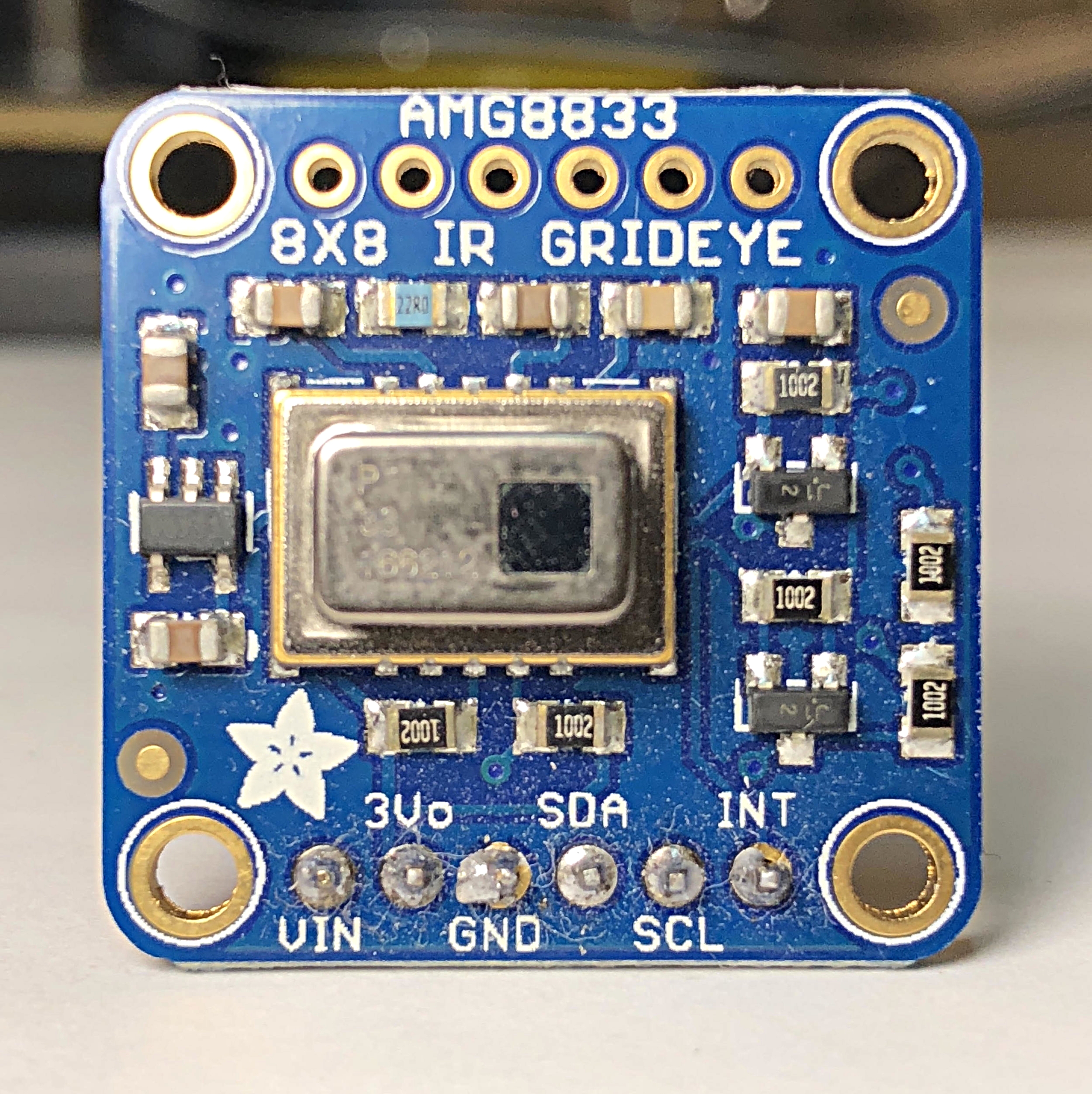
Figure 2: Adafruit's AMG8833 breakout board. This module makes it easy to go from sensor to application with just a few solder points.
The AMG8833 passively measures heat radiation from an infrared-emitting grey body. The temperature is calculated by employing the Stefan-Boltzmann law:
where ε is called the emissivity (between 0 and 1), A is the surface area, σ is the Stefan-Boltzmann constant, T is the temperature of the body, and Π is the radiative power. Typical infrared thermometers (thermopiles of thermocouples) measure radiative power, so there is a conversion needed to approximate temperature. A simple equation for approximating temperature of a grey-body is as follows:
where the V abov represents the voltage measured by the raw sensor. The variable k is an empirical constant that absorbs the A, ε, σ and electronic noise that may exist. The Ts is the temperature of the sensor itself, and the remaining Tobj is the temperature of the object being measured. The sensor temperature is being subtracted to ensure that the temperature of the sensor is not biasing the object temperature measurement. In order to arrive at an accurate prediction of temperature, these sensors are often calibrated using the target material at different temperatures to ensure the value of k is accurate. And once this is done, an empirical equation for object temperature can be implemented:
And this equation is the 'final' approximation for determining temperature of a grey-body using an infrared detector (see full procedure done here).
Parts Description and Wiring
The two principal components used for this project are the Raspberry Pi Zero W ($10, at Adafruit) and the AMG8833 breakout board ($60 from our store). I know the $40 IR sensor seems pricey, but its capabilities far outweigh the cost. As far as I know, there isn't any other multi-pixel IR detector near this price and abundance apart from the Omron D6T series, which is more expensive and boasts a mere 16-pixels (D6T datasheet here). The Raspberry Pi Zero W is used because of its affordability, proficiency, and low profile. I wanted the footprint of this project to be minimal so that the application would be realizable. Minimal tech designs from the start adapt into sleek products. Think of any smart device today - there are components packed into every corner to optimize the user experience.
The AMG8833 also uses I2C to communicate with the Pi. This is great because it only uses two pins on the Pi and the wiring is simpe! The data transfer rate is quick as well, so there is no concern of lag between component performance and reading data into the Pi.
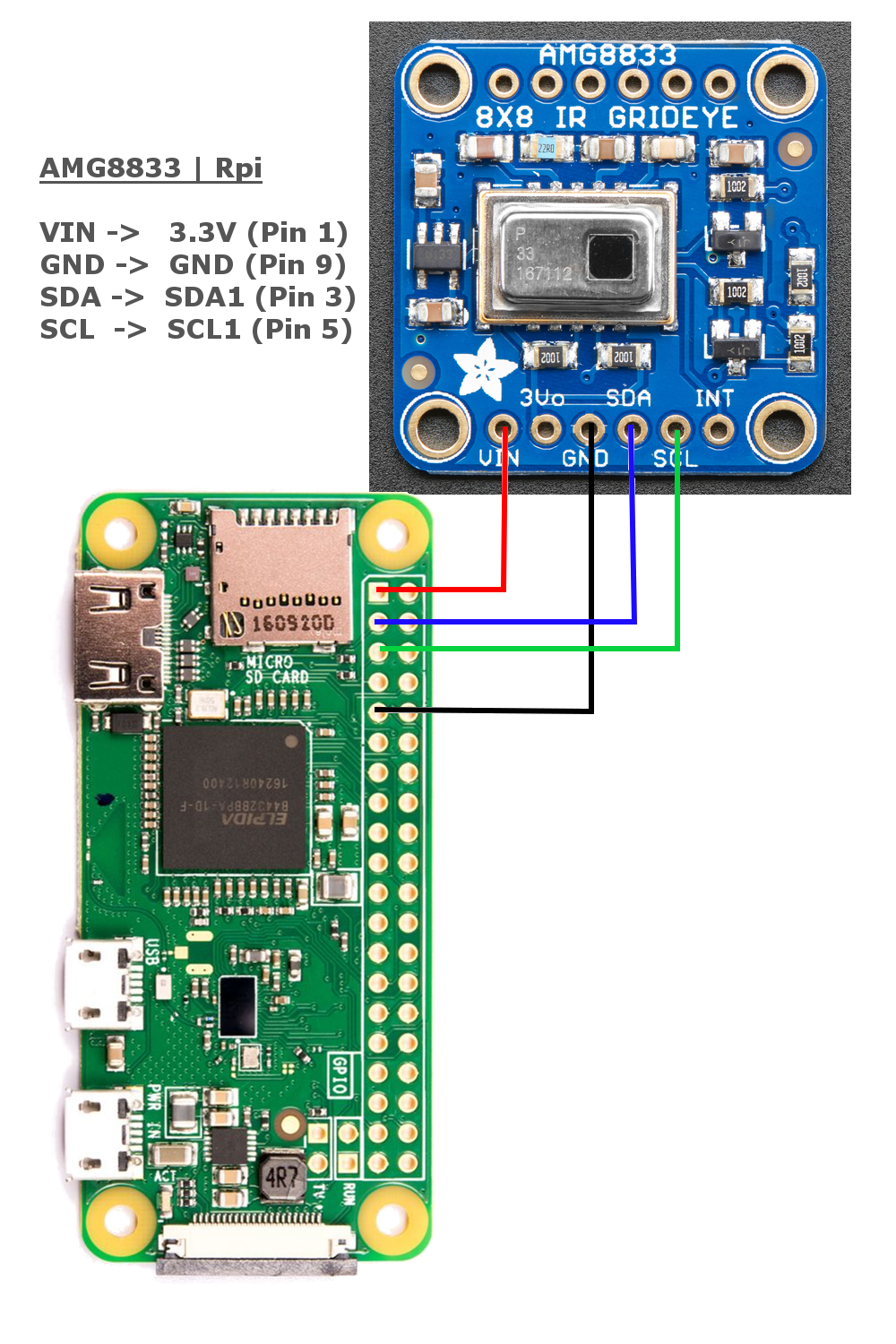

Figure 3: AMG8833 (left) and Raspberry Pi Zero W (right) are the principal components for this project.
---- AMG8833 ----
- 64-pixels (8x8 grid)
- 10 Hz data rate
- I2C fast acquisition
- 4.5 mA power consumption (average)
- ± 2.5°C Accuracy
- Detection distance up to 7 m
These features, along with the performance of the Rpi Zero W give a data update rate around the 10Hz AMG8833 sample rate. Therefore, we are capable of reading nearly 640 data points every second. In actuality, due to issues I will discuss below, the update rate is closer to 1.6 seconds because of the graphics requirements from the Python plotting tool, however, this is only due to the limitations of the RPi, not the sensor. If you want to read a full briefing of the capabilities and applications of the AMG8833 sensor, see this great resource.

We also have an AMG8833 available in our shop
Smaller form factor, with the same functionality
Python Code and Adafruit's AMG88xx Library
The data analysis section of this project is perhaps the most difficult and involved. Nevertheless, I chose Python as the programming language because of its vast data processing toolbox and the existence of an AMG88xx library. The AMG88xx library handles the I2C protocols and returns the temperature values of the 64 individual IR detectors, which aleviates a lot of unnecessary work on the signal processing end. We will still need to conduct normalization prcessing to get a clean signal without the interference of the environment, and I will discuss how I did this below.
The code below is the complete Python script needed to plot a live heat map on the Raspberry Pi. Assuming the AMG8833 library is installed, the devices are wired correctly, and the RPi is configured for I2C - everything should work correctly. From here, I will break down pieces of the code so that the user can understand my methods and eventually alter them to support a specific outcome.
#!usr/bin/python
import sys
import os.path
sys.path.append(os.path.join(os.path.dirname(__file__),'..')) # this is done for the AMG88xx folder (you may have to rewrite this to include the path of your AMG file)
from Adafruit_AMG88xx import Adafruit_AMG88xx
from time import sleep
import time
import matplotlib as mpl
mpl.use('tkagg') # to enable real-time plotting in Raspberry Pi
import matplotlib.pyplot as plt
import numpy as np

sensor = Adafruit_AMG88xx()
# wait for AMG to boot
sleep(0.1)

# preallocating variables
norm_pix = []
cal_vec = []
kk = 0
cal_size = 10 # size of calibration
cal_pix = []
time_prev = time.time() # time for analyzing time between plot updates

plt.ion()

try:
        while(1):
                # calibration procedure #
                if kk==0:
                        print("Sensor should have clear path to calibrate against environment")
                        graph = plt.imshow(np.reshape(np.repeat(0,64),(8,8)),cmap=plt.cm.hot,interpolation='lanczos')
                        plt.colorbar()
                        plt.clim(1,8) # can set these limits to desired range or min/max of current sensor reading
                        plt.draw()
                norm_pix = sensor.readPixels() # read pixels
                if kk<cal_size+1:
                        kk+=1
                if kk==1:
                        cal_vec = norm_pix
                        continue
                elif kk<=cal_size:
                        for xx in range(0,len(norm_pix)):
                                cal_vec[xx]+=norm_pix[xx]
                                if kk==cal_size:
                                        cal_vec[xx] = cal_vec[xx]/cal_size
                        continue
                else:
                        [cal_pix.append(norm_pix[x]-cal_vec[x]) for x in range(0,len(norm_pix))]
                        if min(cal_pix)<0:
                                for y in range(0,len(cal_pix)):
                                        cal_pix[y]+=abs(min(cal_pix))

                # Moving Pixel Plot #
                print(np.reshape(cal_pix,(8,8))) # this helps view the output to ensure the plot is correct
                graph.set_data(np.reshape(cal_pix,(8,8))) # updates heat map in 'real-time'
                plt.draw() # plots updated heat map
                cal_pix = [] # off-load variable for next reading
                print(time.time()-time_prev) # prints out time between plot updates
                time_prev = time.time()

except KeyboardInterrupt:
        print("CTRL-C: Program Stopping via Keyboard Interrupt...")

finally:
        print("Exiting Loop")
Adafruit's AMG88xx library is imported above along with matplotlib (a plotting tool), and numpy (an analysis tool). The first important lines of code are those indicating the plotting methods used:
graph = plt.imshow(np.reshape(np.repeat(0,64),(8,8)),cmap=plt.cm.hot,interpolation='lanczos')
plt.colorbar()
plt.clim(1,8) # can set these limits to desired range or min/max of
current sensor reading
plt.draw()
The code above arranges the 64 temperature readings in an image array distributed in an 8x8 grid. Python then interpolates the data by using the 'lanczos' method. This method is essentially a windowed sinc function, but the important part is that this particular interpolation demonstrates the best results for heat mapping (in my opinion). In the code above, we also request a colorbar, set limits on the temperature, and ask the program to draw the plot immediately.
Following the above code, we move to the environmental normalization procedure:
for xx in range(0,len(norm_pix)):
        cal_vec[xx]+=norm_pix[xx]
        if kk==cal_size:
                cal_vec[xx] = cal_vec[xx]/cal_size
Above we are normalizing the sensor to the environment. I chose to do this because I wanted the environment to have almost no impact on the measurements I was going to make. Note: this method I have chosen will not give readings of temperature, but rather the temperature above the environment when the sensor is being calibrated with the surroundings. If you want to approximate temperature fromm this, I suggest placing an object of known temperature and emissivity near 1 in front of the sensor and calibrate each pixel that way. The method I am using is designed to measure changes in IR radiation.
In the next bit of code, I ensure no negative values are present in the plot because this will introduce erratic results during plotting. I counter this by adding the lowest negative value to each pixel - this will give us an absolute reference frame to indicate heat intensity.
[cal_pix.append(norm_pix[x]-cal_vec[x]) for x in range(0,len(norm_pix))]
        if min(cal_pix)<0:
                for y in range(0,len(cal_pix)):
                        cal_pix[y]+=abs(min(cal_pix))
Finally, the last piece of code updates the plot with the new interpolated pixels by using the method: 'graph.set_data()' - I also included a few lines with printouts of time between loops and the calibrated pixels, just in case you want to view the pixels and ensure what you're seeing on the plot is what you're seeing printed in the terminal.
graph.set_data(np.reshape(cal_pix,(8,8))) # updates heat map in 'real-time'
plt.draw() # plots updated heat map
cal_pix = [] # off-load variable for next reading
print(time.time()-time_prev) # prints out time between plot updates
time_prev = time.time()
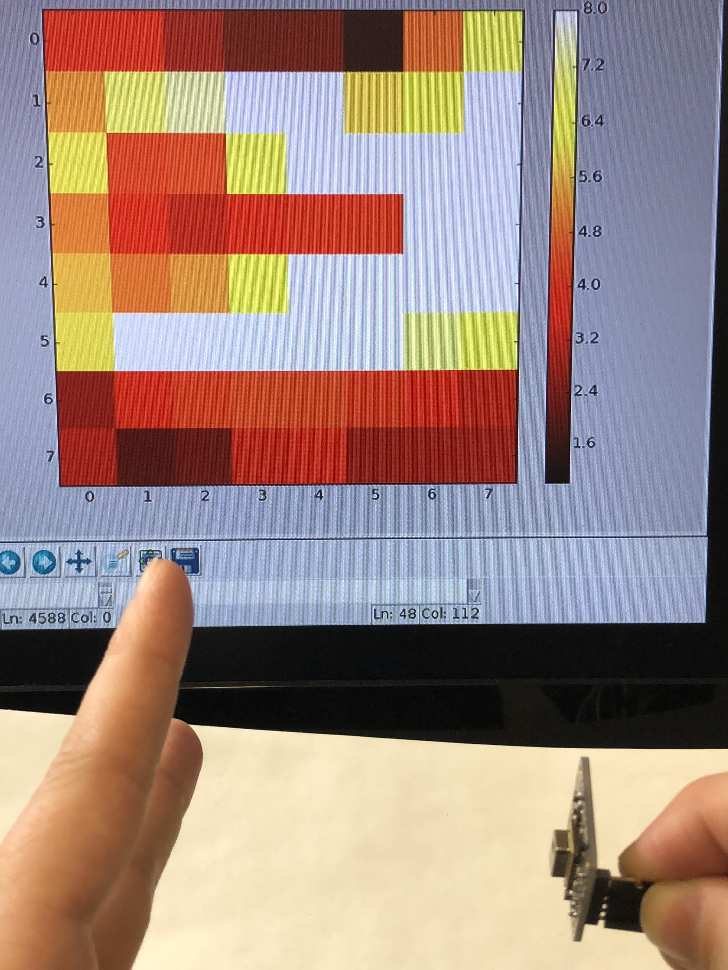
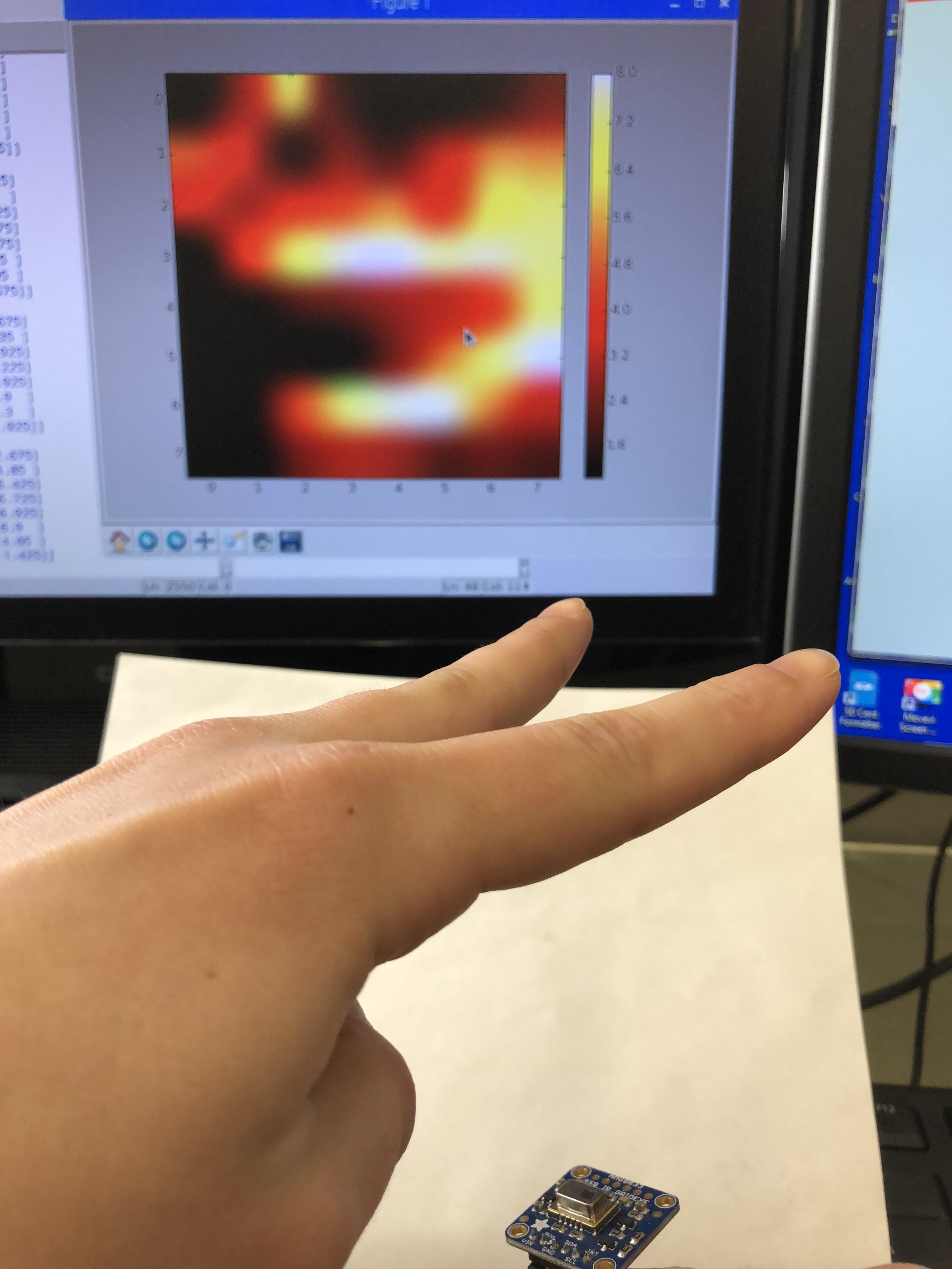
The final lines of code are only for cleaning up the program after exiting (using CTRL-C). I used a 'try' method to ensure that any errors will close the program successfully. This marks the end of the code, and I will be assuming henceforth that the user was able to reproduce the code above and was able to acquire data and plot the relative heat map values using the AMG8833 and Pi in Python. I will only use the simple code above to visualize a heat map of my fingers. This makes understanding the output much easier: the dark regions represent cooler areas (or normalized areas to the background), and the more yellow and whiter regions indicate a hotter source, such as a finger or hand. I used the interpolation format ('lanczos') because I wanted to resolve individual fingers; and upon investigation of the plots below - I was able to do just that.
Results
At this point, you should have a working heat map using the AMG8833 and Raspberry Pi. Below are two photos of my experimentation with the code and IR detector. On the left, I set the interpolation method to 'none' to view the raw pixels. As you can see, the raw values represent two fingers reasonably well. On the right is the implementation of the 'lanczos' interpolation method, and it is easy to observe the improved results compared to the same two-finger heat map on the left.
I also filmed a video below to demonstrate that the sensor and interpolation procedure are capable of resolving THREE fingers at a nearby distance. It is also observable that there is a significant time delay in the heat map. This is a result of the graphics utilization of Python and the limitations of Raspberry Pi. Here, I am able to resolve 1 snapshot every 1.5 seconds depending on the interpolation method. This is in stark contrast to the 10 Hz resolution of the raw values. Conversely, if I do not plot the data the sample rate returns to the near 10 Hz, indicating that the issue is with RPi and its processing limitations, not the I2C support. This type of graphics shortcoming is common for the Raspberry Pi Zero W, as it is not necessarily developed for intense graphics processing.
Conclusion And Discussion
One major takeaway from this experiment is that technology is moving at a rapid pace. It is remarkable that for $50, anyone with minimal programming skills and basic electronics knowledge is capable of building a 64-pixel infrared camera. That being said, this project was intended to be part programming and part engineering, and thus, I am disappointed in the inflexibility of the AMG8833 temperature calculation procedure. The closed calculation limits the user's educational gains regarding heat production, the infrared spectrum, and grey-body radiation. Fortunately, the simplicity of the temperature output made the Python and programming section of this entry much easier. I stated at the beginning of this project that the goal was to educate the user on heat mapping and data analysis tools, and I was certainly able to achieve both of those by using the intuitive approach of human body heat and background normalization.
Upon further exploration of the IR heat map results above, one may discover several difficulties regarding time resolution. This is absolutely a limitation of the Raspberry Pi and the cumbersome nature of the Python graphics requirements. This is why, without plotting the data, the data rate is almost 10 Hz, but the real-time plot data update changes to one point every 1.5 seconds. This may be an issue for someone trying to display high-speed heat maps in real time, but I recommend saving the data in real-time and then plotting the heat maps after the data collection procedure. This will give the illusion (at the maximum 10 frames/sec) of a high-speed 64-pixel heat map.
We love the AMG8833 sensor because of its raw engineering capabilities. An 8x8 gridded thermometer at a reasonable price is truly a gift to electronics makers. The sensor is in a class of its own, and anyone with enough procifiency and ingenuity could dream up applications ranging from advanced human detection, night vision, materials testing, and even smart home automation. The possibilities are endless, and my hope is that after reading this tutorial someone endeavors to create something original and inspiring. Ultimately, this project serves only as a glimpse into the world of heat mapping and data visualization, and is an even tinier examination of thermal radiation. I enjoyed this project so intensely that am determined to return to this project with a different application - so stay tuned and I will update as the project unravels!
See More in Raspberry Pi and Engineering: