Infrared Thermometry Theory and Applications with Arduino and Python
“As an Amazon Associates Program member, clicking on links may result in Maker Portal receiving a small commission that helps support future projects.”
At the turn of the 20th century, scientists began discovering laws that state the wave-like nature of light, something that was foreign to the physics community at the time. Max Planck was a particularly important physicist that was able to use his knowledge and experience with thermodynamics and the burgeoning fields of electromagnetics and radiation to derive a relationship between wavelength of light and temperature. Planck won the Nobel Prize in Physics in 1918:
“in recognition of the services he rendered to the advancement of Physics by his discovery of energy quanta.”
Planck’s discovery of energy quanta and their relationship to thermodynamics is the basis for radiation detectors and infrared temperature sensors. We will use Planck’s law to derive a usable equation that can relate the radiation measured by an infrared sensor to the temperature of a radiative object.
In this tutorial, I will explore black body radiation, infrared detectors, and the relationship between temperature and emissivity - all with the intention of exploring how infrared (IR) detectors measure temperature from a distance. Arduino will be used, along with an MLX90614 IR thermometer, and a thermocouple for true-temperature approximation of each object.

Photo of Max Planck, Courtesy of: https://www.sciencesource.com/archive/Max-Planck--German-Physicist-SS2444907.html
Planck paired his newly-discovered quantum energy theory with thermodynamic relationships to derive an equation for radiation emitted by a perfect “black body” as a function of temperature and wavelength (frequency) of light. The radiation for the body is traditionally given as a function of frequency and temperature:

written in wavelength form:

where:
Bλ (λ,T) ≡ Spectral radiation density [W·sr-1·m-3]
Bν (ν,T) ≡ Spectral radiation density [W·sr-1·m-2⋅Hz-1]
h ≡ 6.62607015×10⁻³⁴ [J · s] (Planck's constant )
c ≡ 299,792,458 [m · s-1] (speed of light)
λ ≡ Wavelength of light [m]
ν ≡ frequency of light [Hz]
kB ≡ 1.380649 × 10⁻²³ [J⋅K-1 ] (Boltzmann's constant)
T ≡ Temperature of body [K]
A derivation of Planck’s law can be found at Radiative Processes in Astrophysics by Harvard-Smithsonian Center physicists George B. Rybicki and Alan P. Lightman. Page 20 contains the full derivation.
Radiation can be plotted as a function of wavelength and temperature using the Planck law:
We can see very specific behavior in the plot above, mainly, that an increase in temperature results in an increase in radiation emission. We can also deduce that each wavelength emits differing amounts of radiation based on temperature. This conclusion was crucial for understanding a multitude of phenomena observed in physics, for example the photoelectric effect and correlation photodetectors and temperature, which we will use later in this tutorial.
Now, if we look at the more relevant temperatures to every-day life, we can see how radiation emission amplitude and peak both change with decreased temperature:

Notice in the above, the amplitude of the spectral radiance is much lower than at the higher temperatures. There is also a shift in wavelength peak for radiation. We can broaden the wavelength range and adjust the normalization of the radiation term to get a clearer picture of what’s happening:
The relation above is often integrated to approximate the radiation of an object over a range of wavelengths. This integration can then be used to approximate temperature based on the response of a particular sensor. This integration is written as:

where:
The radiation density is the total energy radiated over a surface at a given solid angle (steradian), which is why we have Watts per square-meter, steradian. We can further integrate over the radiating surface area and solid angle, however, we will leave that for later. The integration was carried out for all wavelengths by Stefan and Boltzmann:

The integration is quite involved and has been carried out here: https://ntrs.nasa.gov/archive/nasa/casi.ntrs.nasa.gov/19680008986.pdf, the basics of involve a substitution and some advanced calculus tricks, but the result gives the following relationship:

where σ is the Stefan-Boltzmann constant, defined as:
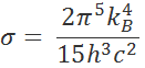

And the result above is one of the most important relationships in modern physics. It states that the emission of radiation at all wavelengths is proportional to the fourth power of the temperature of the object. This result will be crucial for approximating temperature using our infrared sensor.
Python code is given for replicating the plots above:
import numpy as np
import matplotlib.pyplot as plt

plt.style.use('ggplot')

h = 6.6260715*np.power(10,-34.0) # Planck's constant
c = 2.99792458*np.power(10,8) # speed of light
k_B = 1.380649*np.power(10,-23.0) # Boltzmann's constant

# parameters lambda, T
lambda_array = np.arange(0,4010,10)
##T_array = np.arange(250.0,420.0,10) # uncomment for lower range of T
T_array = [1000,2000,3000,4000,5000]

fig,ax = plt.subplots(figsize=(12,8)) # figure for plotting in loop
for T in T_array:
    B_T_array = []
    for lambda_nm in lambda_array:
        B_0 = 2.0*((h*(c**2))/np.power(lambda_nm*np.power(10,-9.0),5.0))
        B_exp_0 = (h*c)/(k_B*np.power(10.0,-9.0))
        B_T = (B_0/(np.exp((B_exp_0/(lambda_nm*T)))-1.0))
        B_T = ((B_T)/1000.0)*np.power(10.0,-9.0)
        B_T_array.append(B_T) # radiation for wavelengths at T
    ax.plot(lambda_array/1000.0,B_T_array,label=' K'.format(T),linewidth=4)

# setting axis parameters
ax.set_xlim([lambda_array[0]/1000.0,lambda_array[-1]/1000.0])
ax.set_ylabel(r'Spectral Radiance [kW sr$^$ m$^$ nm$^$]',fontsize=16)
ax.set_xlabel('Wavelength [$\mathrm$m]',fontsize=16)
ax.legend(fontsize=14)
ax.tick_params(axis='both',labelsize=14)
plt.show()
The relationship between radiation and temperature above is for the perfect black body. However, it is nearly impossible to achieve a perfect black body, so the introduction of grey bodies facilitates the real-world application of Planck’s theory and black body radiation. In order to be considered a grey body, the radiation emitted from an object must be less than that of the perfect black body with the same dimensions. This relationship is called emissivity:

where ε is the emissivity, qb is the radiation emitted by a black body, and qg is the radiation emitted by a grey body. Under these assumptions, ε is always less than 1.
A perfect black body absorbs all the incident radiation, allows none to reflect off its surface, and does not allow transmission through its surface. This can be written as follows:

where α represents the absorption of the incident radiation, τ is the transmission of radiation into the body, and ρ is the reflected amount of radiation. For a black body, we know that there is no reflection or transmission, which is not the case for a grey body. Below is the radiation balance for a given grey body:
Most grey bodies encountered are opaque and so we can ignore the transmission of radiation as well, resulting in the very simplified radiation balance:

Kirchhoff’s law of thermal radiation states that:

which allows us to write the final equation for grey body radiation balance as a function of its ability to emit radiation close to that of a black body:

This result will be important for determining the amount of reflected radiation for different materials, allowing us to make assumptions about materials and temperature based on the Stefan-Boltzmann law.
Infrared thermometers are contactless temperature sensors that harness many of the principles derived and given above. They use the Stefan-Boltzmann law to relate the amount of radiation incident on the sensor to the temperature of the object emitting radiation. Then, the radiation is coupled with some grey body assumptions based on the material of the object being measured. These principles, along with some clever balances and electronics can be used to relate the voltage read from a sensor to the approximate temperature of an radiative object.
First, we need to setup the bounds of the non-contact temperature system:
The object must be treated as a grey body
The grey body assumption requires the knowledge of emissivity for every object temperature to be measured. There are many tables of emissivity values available online, however, for most laboratory procedures, the emissivity must be approximated using a thermocouple or other reliable temperature measurement.
Radiation sensors are band-limited
Band-limited refers to the fact that the sensor will not measure an infinite amount of wavelengths. This will need to be addressed by altering the integration of the Planck equation.
Background radiation can contaminate the sensor readings
It is customary to take ambient temperature measurements to reduce the interference of background radiation.
There is a widely cited publication called “Infrared Thermography for Temperature Measurement and Non-Destructive Testing” by Ruben Usamentiaga et al. that elaborates upon these complications and the implications that arise when dealing with non-contact temperature sensing. The publication can be found here:
https://www.ncbi.nlm.nih.gov/pmc/articles/PMC4168422/
The authors cite a simple balance of radiation to account for atmospheric effects as well as the radiation from the body itself. A drawing of the theoretical radiation balance is shown below:
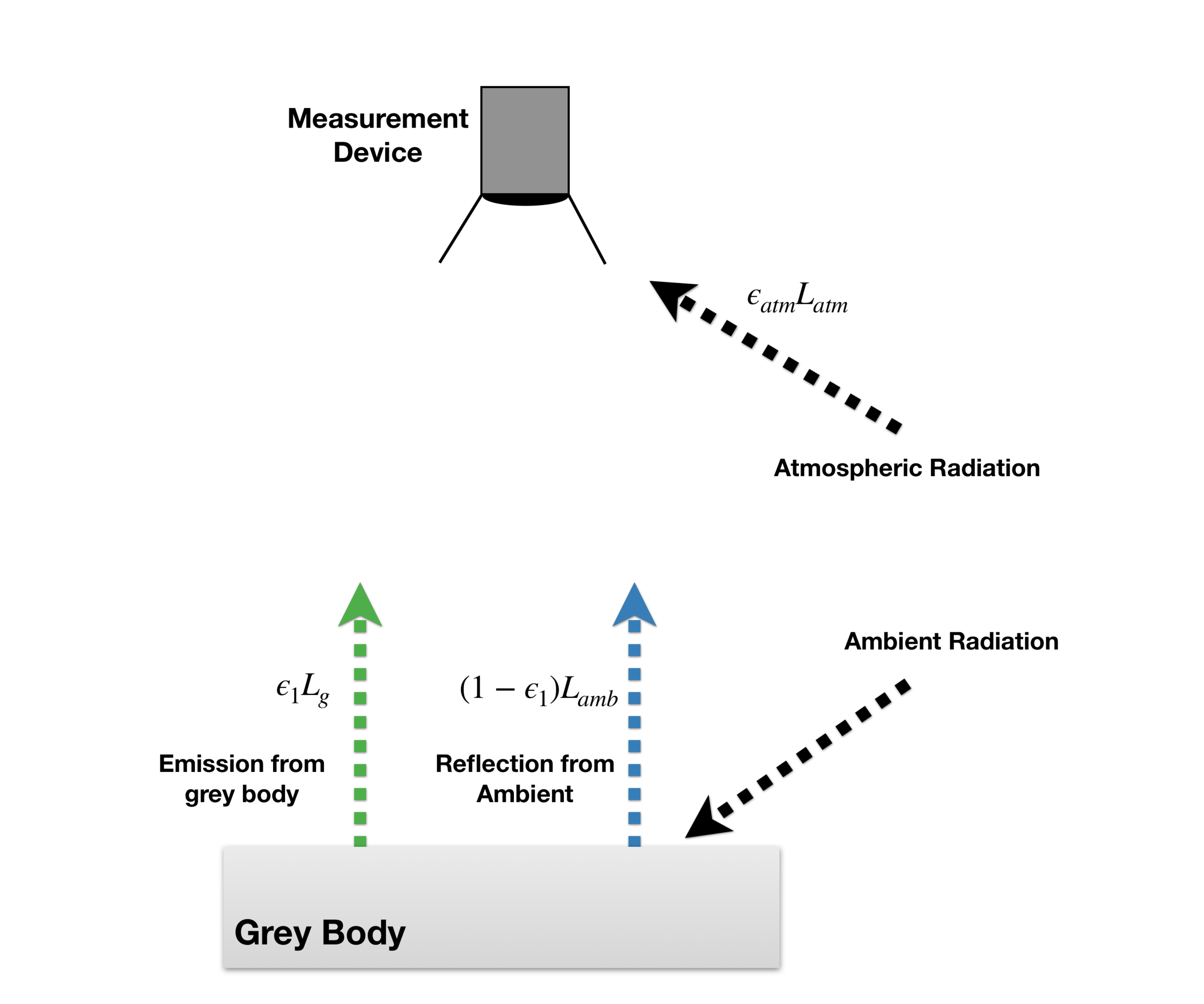
The radiation measured by a sensor pointed at an emissive object is given below using a radiation balance:

where Lnet is the net radiation density incident on the sensor, Lobj is the radiation emitted by the object, Lref is the reflected ambient radiation of the surrounding area (other raditing objects), and Latm is the direct radiation from the atmosphere. The direct radiation from the atmosphere for most applications over short distances is negligible, so the emissivity associated with atmospheric radiation is usually zero; and thus, it is ignored here.
Implementing the paramters from the figure above, we can write the final net radiation balance:

This is a simplified model that is used for measuring object temperatures with a close-proximity sensor. The emissivity, ε1, is the emissivity of the object material. Lg is radiation of the object were it a perfect black body, and the reflected radiation uses the radiation of a black body associated with the ambient radiation, Lamb, multiplied by the reflectivity (1-ε1).
The difficulty of defining Lnet and the other radiation terms lies in the complexity of the sensor. The simplest way to define the net radiation density experienced by the sensor is to assume that the sensor has some absorptivity associated with its radiation detector. This can be written as:

The above uses the emissivity of the radiation sensor itself (which is usually very close to 1). However, in practice many of the parameters associated with the sensor (assuming they are constant) are lumped into one ‘device constant’ that is solved-for using a regression algorithm during calibration.
The final approximation for a non-contact radiation sensor uses the following relationship:

where C0 handles many of the device-specific parameters such as: device surface area, sensor emissivity, viewing angle and other variables that can be lumped-in during site-specific calibrations.
In the field of non-contact temperature measurement, many of the sensors consist of the setup outlined above where the sensor is sensitive to infrared wavelengths. For the sensor that will be used in this tutorial, the range of wavelengths is form 5.5 µm - 14 µm, which is slightly in the red visible band and over in the near infrared range. If we go back to the Planck equation, we can see just how we might integrate over the finite band:

If we make a substitution and pull out some of the constants from the integrand:


The integral above tells us a few things:
- The radiation measured by the sensor is still a function of T4 over the limited wavelength range
- Band-limited radiation will need to be numerically integrated
- As more wavelengths are added to the integral, we approach the Stefan-Boltzmann relationship
The problem just became very difficult because of the temperature-dependent integration. But this does not mean we are without solutions!
If we plot both the Stefan-Boltzmann relationship and the numerical finite-wavelength integration, we can see how they compare:

It is clear from the figure and predicted by theory that as we add more wavelengths to the integration, we approach the Stefan-Boltzmann relationship. Since our sensor wavelength band is from 5.5 µm - 14 µm, we can deduce from the plot above that the Stefan-Boltzmann relationship will not be valid for our calculations. Fortunately, the relationship is not overly complex, so we can create a relationship between our wavelength temperature profile and the Stefan-Boltzmann curve.
For the particular case of our infrared sensor, the ratio of Stefan-Boltzmann radiation to our band-limited radiation is as follows:

If we return to the radiation balance above and write it in terms of the Stefan-Boltzmann radiation, we can see how temperature emerges from radiation:

where again the constant C0 encompasses several sensor-specific or site-specific parameters. The sensor radiation term accounting for the band-limited correction is given as:

which we can use to correct the radiation balance above:

We now face the problem of handling the f(T) terms, which in most cases are assumed to be 1, and therefore can be ignored. However, if we want to ensure our limited-bandwidth sensor is accurate over large temperature ranges, we use a polynomial fit to minimize the error to less than 3% over standard but large temperature ranges (250K - 500K). In most applications, Tamb is measured with a separate sensor, the infrared sensor produces a form of Lsensor/C0, and the object temperature is solved-for as a biquadratic equation, which assumes the following form:

if we remember the polynomial fit terms:

we can explicitly write the biquadratic as a function of Tobj :

which we can collapse into an analysis-ready format:

where the terms are defined as:
b ≡ d2

The coefficients d1,2,3 are all defined based on the polynomial fit of the ratio between band-limited Planck radiation and the Stefan-Boltzmann relationship (given in the Figure above).
A biquadratic equation is defined as:

which has solutions:

This equation will be essential for calculating the resulting temperature correction from our sensor, based on the band-limited response of the sensor compared to the Stefan-Boltzmann relationship.
The equation for temperature above acts under the assumption that the emissivity of the object is known. Calibration should precede any measurements with a device, especially when dealing with sensitive readings from non-contact temperature sensors. Often, thermocouples are used as the calibration point for IR contactless sensors, and so we can setup a method for determining the emissivity using the radiation balance above, though most approximations assume that f(T) = 1:

Solving for ε1:

For many sensors, the raw radiation value is not known, or the value of Lsensor/C0 is unknown. This issue can be resolved by setting the emissivity at an incorrect value, calculating a calibration Lsensor/C0, and then solving for the true ε1. We can setup a two emissivity (one right, one wrong but set) relationship with the Lsensor/C0 values equated:


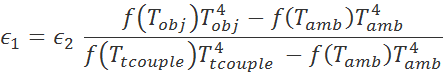
Under the assumption that the sensor readout doesn’t change during calibration and that the true temperature readout is measured by a thermocouple, we can treat ϵ1 as the true emissivity and ϵ2 as the set emissivity. Finally, equating the two values for Lsensor/C0 and solving for ϵ1:

This is an important result in that it uses three temperature measurements and a set value for emissivity to calculate the true emissivity of the object material.
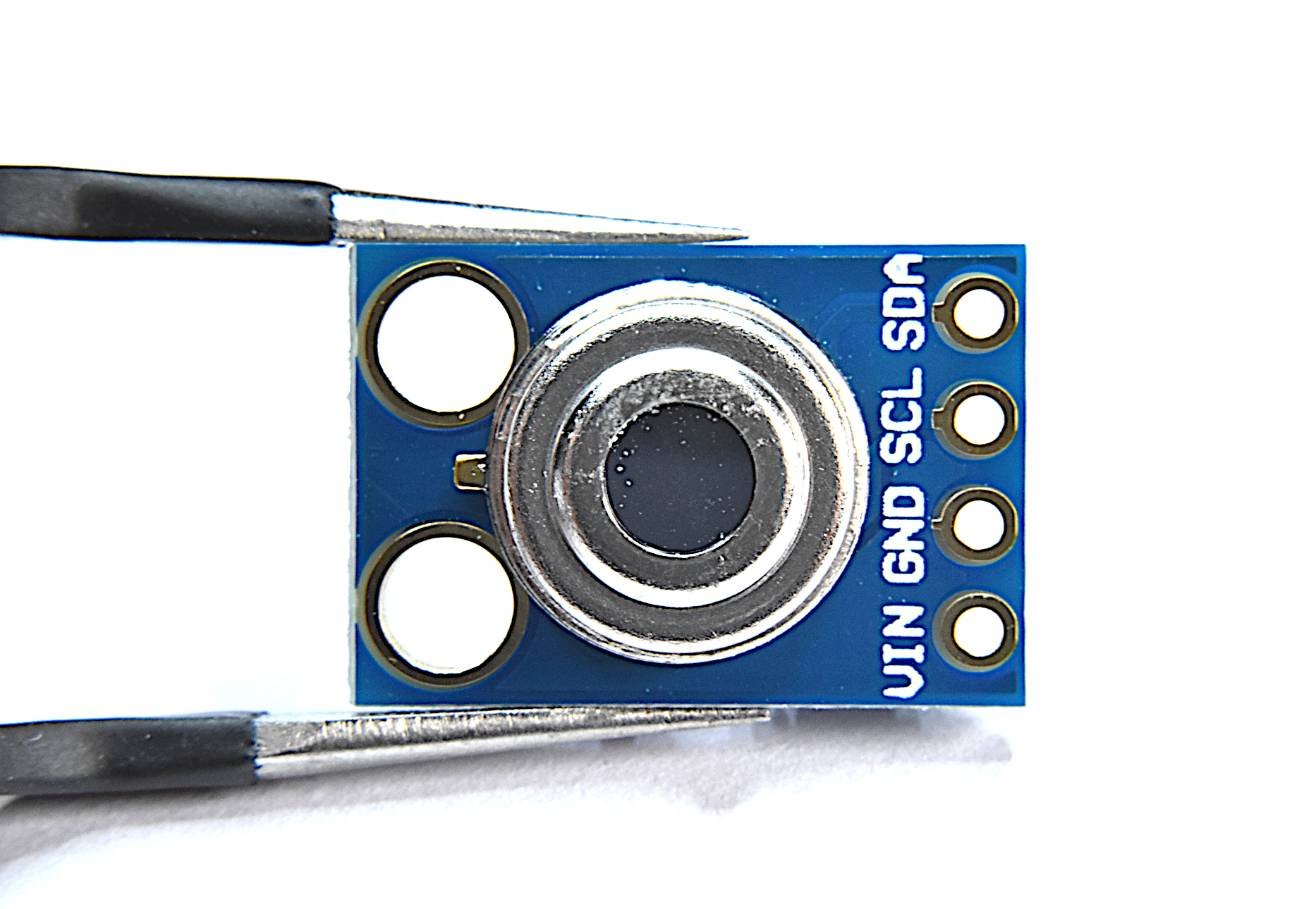
The MLX90614 is a band-limited infrared sensor that uses many of the techniques discussed above to approximate temperature as a function of radiation and material emissivity. The MLX90614 allows the user to change the emissivity, but it does not allow you to record raw radiation data (or radiation as a function of voltage). This makes things difficult for customization and testing, however, we can perform some tests to back-out their algorithm and test whether we can improve their algorithm and verify some of the formulas given above. The datasheet for the MLX90614 is given over at Sparkfun. There is minimal information regarding their algorithm used to approximate temperature (only a mention of the Stefan-Boltzmann for object and ambient temperature) - so we will have to reverse engineer a lot of the sensor inputs and outputs.

Using the MLX90614 and a thermocouple to measure temperature of a heated block of wood.
PARTS LIST:
The basic setup for the experiments is given in the image above, as well as a wiring diagram for Arduino below. The parts used in this experiment are also given:
The wiring diagram for each component and the Arduino board is given below:
A table with each pinout is also given below:

Finally, the sample code to be used in Arduino is given. It prints out a timestamp in milliseconds, the object temperature for the thermocouple, the object and ambient temperature from the MLX90614, and the ambient temperature and humidity from the DHT-22 sensor. The code also puts the used emissivity into the last column of the printout. I recommend using Python or a datalogging program to record the printout of the temperature data, to be used for analysis.
#include <SPI.h>
#include "Adafruit_MAX31855.h"
#include <Wire.h>
#include <SparkFunMLX90614.h>
#include "DHT.h"

// Example creating a thermocouple instance with software SPI on any three
// digital IO pins.
#define MAXDO   3
#define MAXCS   4
#define MAXCLK  5
#define DHTPIN 2
#define DHTTYPE DHT22
int mlx_pin = 6;
int mlx_gnd = 7;
int dht_pin = 8;
int dht_gnd = 9;

// initialize the Thermocouple
Adafruit_MAX31855 thermocouple(MAXCLK, MAXCS, MAXDO);
DHT dht(DHTPIN, DHTTYPE);
IRTherm therm; // Create an IRTherm object to interact with throughout

int avg_len = 5;

void setup() {
  Serial.begin(9600);

  // pins for MLX control
  pinMode(mlx_pin,OUTPUT);
  pinMode(mlx_gnd,OUTPUT);
  digitalWrite(mlx_pin,HIGH);
  digitalWrite(mlx_gnd,LOW);
  delay(100);
  therm.begin(); // Initialize thermal IR sensor
  delay(500);

  // pins for DHT control
  pinMode(dht_pin,OUTPUT);
  pinMode(dht_gnd,OUTPUT);
  digitalWrite(dht_pin,HIGH);
  digitalWrite(dht_gnd,LOW);
  dht.begin();
  delay(2000);

  print_header();
  therm.setEmissivity(0.5);
  delay(1000);
  Serial.print("NEW EMISSIVITY: ");
  Serial.println(therm.readEmissivity());
  therm.setUnit(TEMP_C);
  Serial.println("program start");
  delay(100);
}

void loop() {
  float thermocouple_t = thermocouple.readCelsius();
  float obj_sum = 0.0; float mlx_t = 0.0;
  float amb_sum = 0.0; float mlx_amb = 0.0;
  float avg_n = 0.0;
  digitalWrite(mlx_gnd,LOW);
  delay(50);
  for (int ii=0;ii<avg_len;ii++){
    bool read_bool = therm.read();
    mlx_t = therm.object();
    mlx_amb = therm.ambient();
    if(read_bool!=false and mlx_t>-70 and mlx_amb>-70){
      obj_sum+=mlx_t;
      amb_sum+=mlx_amb;
      avg_n+=1.0;
    }
  }
  mlx_t = obj_sum/avg_n;
  mlx_amb = amb_sum/avg_n;

  digitalWrite(dht_gnd,LOW);
  delay(100);
  float dht_t = dht.readTemperature();
  float dht_h = dht.readHumidity();

  if (isnan(thermocouple_t) or mlx_t<0 or dht_t<0){

  } else {
    Serial.print(millis()); // time print
    Serial.print(",");

    Serial.print(thermocouple_t); // thermocouple temp
    Serial.print(",");

    Serial.print(mlx_t); // IR sensor obj temp
    Serial.print(",");
    Serial.print(mlx_amb); // IR sensor ambient Temp
    Serial.print(",");

    Serial.print(dht_t); // DHT22 air temperature
    Serial.print(",");
    Serial.print(dht_h); // DHT22 relative humidity

    Serial.print(",");
    Serial.println(therm.readEmissivity()); // print emissivity
  }

}

void print_header(){
  Serial.println("Thermocoup | MLX (Obj) | MLX (Amb) | DHT22 (Temp) | DHT22 (hum %)");
}
If we assume a certain emissivity (I use 0.5 in the code above), we can use that emissivity to calculate the actual emissivity by relating the thermocouple temperature and MLX90614 temperatures with the equation from above:

We can use this emissivity to calculate the true temperature using just the MLX90614 object and ambient temperatures:

And this gives us the general set of equations for calculating object temperature using a thermocouple as a calibration point for material emissivity. It is wise to first calculate the emissivity of a given surface using the thermocouple, then test that emissivity independently and over a range of temperatures. This will ensure repeatability and accurate temperature measurements of a given material.
The experiment that I conducted consisted of heating of a piece of wood, while the MLX90614 was pointed at the wood, the thermocouple was in contact with the wood, and a DHT22 temperature sensor measuring the ambient temperature. A setup of this experiment is shown below:

Two tests were run:
The first test consisted of heating the piece of wood and measuring the temperature from the MLX90614 at an emissivity of 0.5
The second test was run at another emissivity closer to the actual emissivity of wood (0.9)
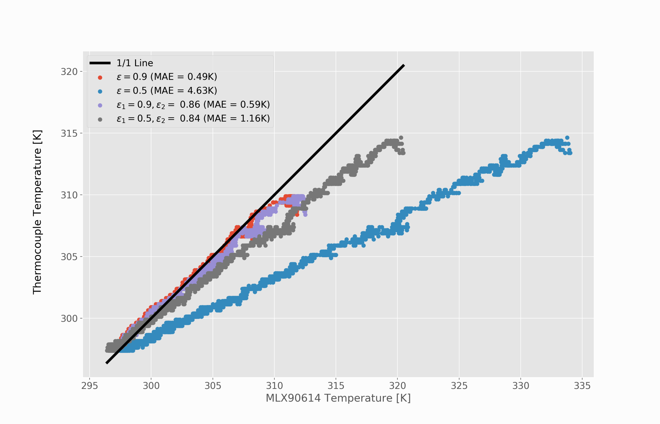
The results are shown below:

In the ideal scenario, each scatter plot should follow the black 1/1 line, where the MLX90614 temperature aligns perfectly with the thermocouple temperature. And we can see, for the most part, the emissivity value of 0.9 roughly leads to this. However, we see that the emissivity value of 0.5 is seriously over-predicting the temperature. To correct this, we can look at our emissivity correction given in the previous section to calculate, using the knowns of the problem, the actual emissivity.
As a measure of the data above we can calculate error for both emissivities:
- (ε = 0.9) Mean Absolute Error = 0.5 K
- (ε = 0.5) Mean Absolute Error = 4.6 K
Implementing the new calculation of emissivity for both:
- (ε1 = 0.9, ε2 = 0.87) Mean Absolute Error = 0.56 K
- (ε1 = 0.5, ε2 = 0.77) Mean Absolute Error = 1.50 K
And we can see how solving for the correct emissivity during calibration is essential for getting the best results (The emissivity also correlates to emissivity values cited at www.infrared-thermography.com)! We can also see that calibration with the correct emissivity is also possible and produces similar results (with slight increase in error in this particular case). The reconstruction of both plots with the correct emissivity is shown below:
This still does not suffice, as there is a deviation in accuracy with increased temperature. Looking back at the finite-band deficit, we can start to correct this drift by realizing the Planckian-corrected emissivity approximation takes the following form:

Returning to our biquadratic equation, we can also define the new object temperature equation:
with the coefficients defined by the fit of the ratio between finite-band and Stefan-Boltzmann radiation:


with the constants in d defined by the polynomial coefficients:


resulting in the final coefficients:


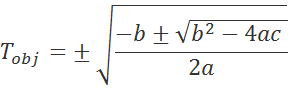
And if we were to conduct some analysis on the Tobj biquadratic equation, we would realize the best selection for positive and real temperatures is:

The only remaining mystery variable is Lsensor/C0 σ, which can be approximated by the initial radiation balance before accounting for wavelength limiting effects:

Where C0 is a constant that will need to be solved-for for the particular sensor in use. For my sensor, it was 2.04. ϵ2 is the emissivity for the original data collection period. Tobj is the temperature approximated from the sensor, and Tamb is the ambient temperature measured by the sensor (usually on-board ambient thermistor or similar) or by an external sensor.
The Planckian corrections for the band-limited IR sensor are shown below in the final plot. The finite-wavelength corrections improved the temperature algorithm by over 4K in the wrong emissivity value readings and improved the temperature prediction by 0.2K for near-correct emissivity. These results indicate that even for normal temperature ranges, accounting for Planckian limited-wavelength sensor radiation can improve temperature readings, specifically when dealing with incorrect assumptions of material emissivity.

From the analysis and results of this experiment, the following statements can be made:
The inverse Stefan-Boltzmann method for finding the emissivity of a material works to lower or maintain the error between thermocouple and non-contact infrared sensor
Non-contact IR sensors show temperature drifting over larger ranges, and therefore must be corrected
The Planck correction for band-limited sensors works to lower the error between thermocouple and sensor by a huge margin (nearly 70% in one case, and 40% in the other)
This was a lengthy exploration of non-contact temperature measurement using an MLX90614 infrared sensor and thermocouple. This project is a multifaceted lesson on physics, engineering, and data analysis. It’s also a mini course on experimentation and calibration. Non-contact temperature sensors have been available and on the market for decades, however, lower quality sensors tend to be inconsistent, not only due to the inexpensive development on the hardware end, but also on the software end. Many of the cheaper IR sensors do not account for limited-wavelength affects from the Stefan-Boltzmann relationship, which can be a problem when measuring large ranges of temperatures. The results of this exploration of IR sensors and Planck’s equation will be helpful for those developing and using band-limited sensors for a multitude of purposes, even outside that of temperature sensing.
See More in Arduino and Engineering: