A Heat Transfer Experiment with Coffee

Few things are better than a shot of espresso in the morning. Following the advent of Nespresso and their streamlined machines, making espresso is easier than ever and the quality has never been better. The excellence of the brand is demonstrated through consistency of both coffee and experience. I wanted to test one of their machines to explore its temperature profile and investigate the optimum drinking period for a given shot. This would help any Nespresso drinker to perfectly time their beverage so as to prevent unwanted cooling and bitterness that often comes from a stagnant brew.

This experiment is often core curriculum for engineering students, especially those interested in fluid mechanics and heat transfer. The measurements support the classical theory of Newton who proposed a fundamental thermodynamic law for convective cooling. This law is known as Newton's Law of Cooling, and it's one of the cornerstones of thermodynamics and the transfer of heat in a fluid.

Nespresso Prodigio and a ceramic espresso mug.

Heat Transfer Background And Experimental Objective

Newton proposed that the time rate-of-change of heat was related to a difference of temperatures and a constant that relates to the fluid's ability to transfer heat. This relation is explicitly stated as: 

where h is the heat transfer coefficient, Q is the heat transferred, A is a characteristic area, T_i is the hot temperature exposed, and T_∞ is the ambient temperature. Using a few thermodynamic laws and assuming a lumped capacitance model (see Jiji text, ISBN: 978-3642012662), we can rewrite the equation in a more experimental-friendly way:

All of the variables remain the same except the new constant, β, which absorbs the heat transfer coefficient, the heat capacity of the fluid (C), and the area of the surface exposed to cooling or heating. The focus of this experiment is to find β, however, we must first find a solution to the differential equation above.

This is a powerful result, because it states that if you start your experiment at a max value, maintain the temperature at the environment, and let time lapse: then you can predict the time it will take to arrive at a desired temperature; or conversely, you can set a time and predict what the temperature will be at that time. So, how do we test and verify this result? In the following section I cover curve-fitting of logarithmic profiles, as well as the experimental setup needed.

---

Experimental Setup

The experimental setup consists of four principal components: 

1. Thermocouple and Max6675 (found here)

2. Arduino Uno

3. Raspberry Pi

4. Hot Coffee or Water (water and espresso used in my experiments)

In the video to the right I show an example of the setup for the experiment. I used the setup on the right to ensure linear effects of the sensor, but I proceeded to use an espresso cup instead of the beeker (because the focus is on Nespresso here). 

Experimental Setup

The tip of the thermocouple goes into the hot beverage, the thermocouple is then wired to the Arduino Uno, and finally the Arduino is connected to the Raspberry Pi where Python collects serial data.

For help with the Max6675 see this Github directory, which is the (un)official library for the device. I used the library for this project, and it really is an out-of-the-box software. Below is my wiring diagram for the setup.

---

Taking Data and Logarithmic Curve Fitting

At this point, we have established enough background and experimental setup to begin taking measurements. Using Python, I recorded the Arduino serial data measured by the thermocouple. The temperature profile is plotted below.

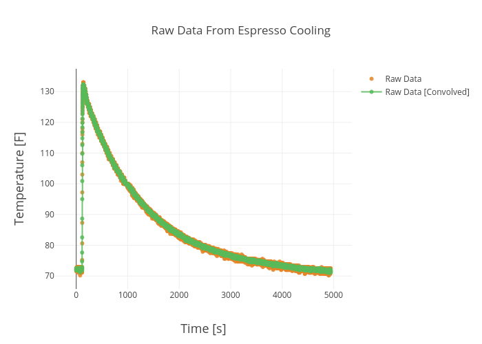
This is the expected trend, first a few points around room temperature, then a spike when the thermocouple is dropped into the hot coffee.The two plots are raw data, but one has been convoluted with a vector of ones in order to lower the noise.

Now, I will cover some basics of curve fitting with Python and exponential functions. To start, we want to rearrange our temperature function to prepare it for polynomial fitting.

Here we can see that our equation has taken the form of slope intercept:  y = mx+b, where b is some error constant that will be determined by the fitting. Also, as usual m is the slop of the line, t is the variable, and y is the expected linear behavior of the logarithm over time. If it is unclear what we are looking for, I suggest reading about polynomial fits and their significance in empirical methods in engineering. 

We wish to find β and ε, so we use Python's fitting tool. After applying the fit to my data, I found the constants:

We can also reconstruct our temperature solution from Newton to look like the following:

Finally, we have a heat transfer solution to our system. The final equation above states that in our espresso system, we can predict the time that it takes for the system to cool to a specific temperature, and we can also predict the temperature of our system at a specified time. This is a classic result that has applications in various fields involving HVAC, aerospace propulsion, and even postmortem evaluation for time of death. Below is the reconstruction that uses the Python fit results - it's easy to see the success of such a simple tool.

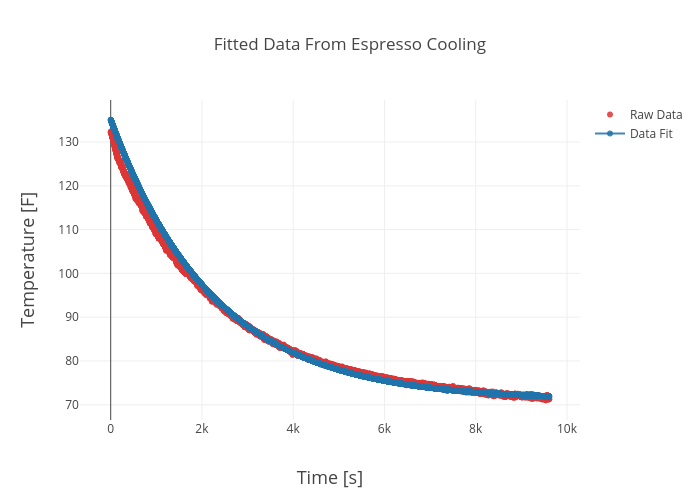
Reconstruction of the exponential profile for the espresso cooling experiment.

This experiment has demonstrated several feats of engineering. First, it established the quality and consistency of the Nespresso machine (I conducted this experiment 5 times and the results were incredibly consistent, for an interesting read on optimization of coffee drinking temperature, see here. Nespresso really nails it.). Second, the inexpensive equipment proved to be more than adequate for this simple experiment. The Arduino, thermocouple, and Raspberry Pi together cost less than $100 and the results compete with instrumentation that far exceeds that monetary minimum. And third, Newton's Law of Cooling was impressively supported by the results of the experiment, as is validated in the reconstruction above.

I sincerely hope that this experiment has endowed a sense of meaningfulness to the symbols and numbers that so often foil one's intuition. Experimentation and validation can serve as ignitions for creativity and exploration; and I hope this sequence has lit someone's spark somewhere.

Related Items from our Shop:

Sold out

Quick View

Maker Portal Arduino-Compatible Uno Rev3 Board

$13.00

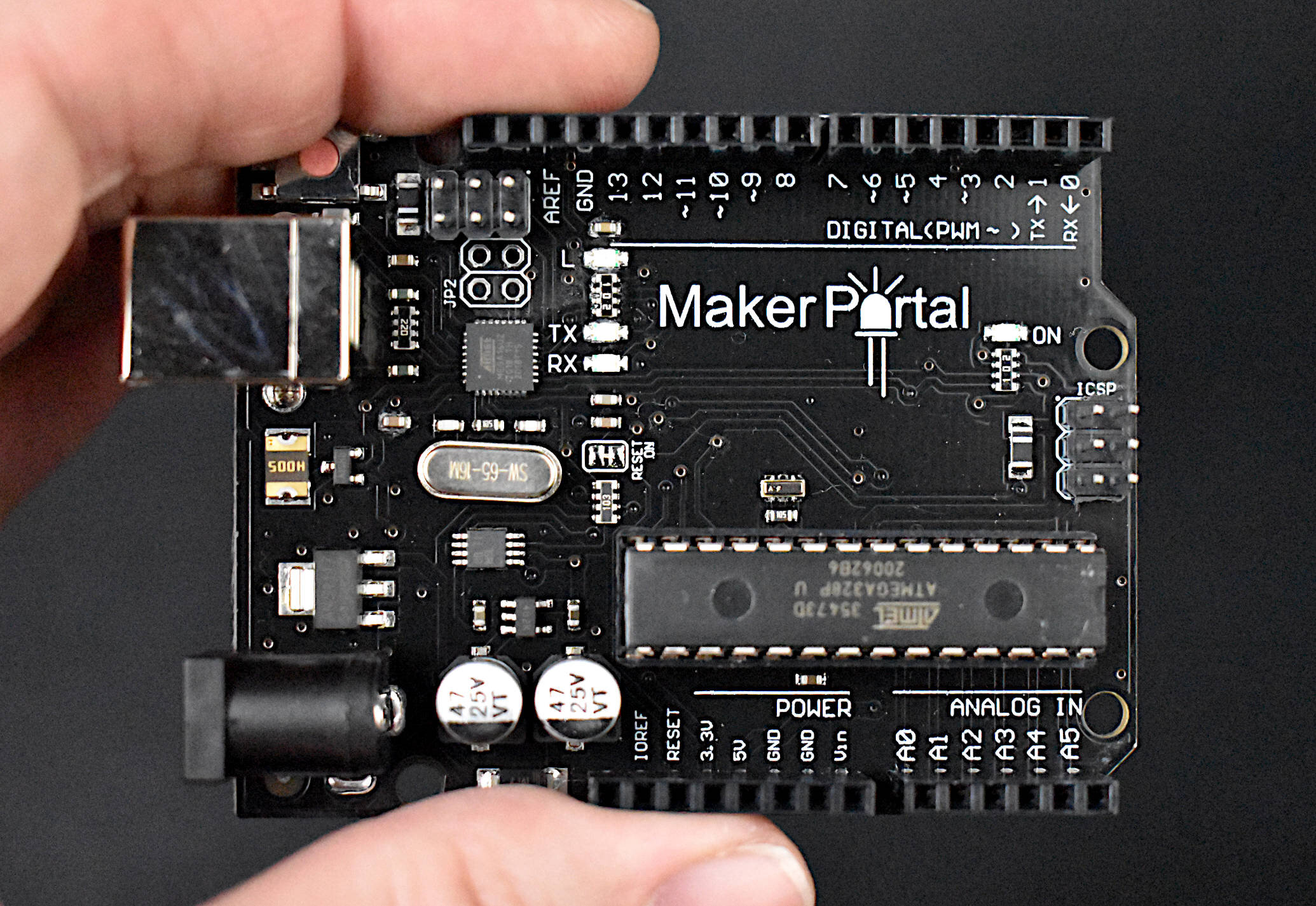
The Maker Portal Uno board is the centerpiece of many of the projects carried out in our maker spaces. The Uno board is capable of reading a wide range of sensors using analog-to-digital conversion, SPI, I2C, UART, and other common protocols. The Uno board can be used to control motors, OLED/LCD displays, and LEDs. The Arduino Uno board shown here is the official Maker Portal microcontroller, which we use in many of our projects!

Included in the Arduino Uno Package:

• Maker Portal Arduino Uno Rev3 Board

• Black USB Cable (1m in Length)

Specifications for Arduino Uno Rev3 Board:

• ATmega328P chip with Arduino Bootloader

• 14 digital pins, 6 analog pins

• 10-bit analog-to-digital converter (ADC)

• 5V-12V Supply Tolerance

• 3.3V and 5.0V output pins

• 16 MHz clock

• 5 PWM pins, I2C support, SPI support , UART support

• ATmega16U2 USB TTL, compatible with Linux, Windows, and Mac

• Black Stylish Finish

• Fully Integrated with Arduino IDE software

Purchase

Sold out

Quick View

K-Type Thermocouple + MAX31855 Amplifier

$12.00

Included in Package:

1. K-Type Beaded Thermocouple

2. MAX31855 amplifier

3. Breakout pins and header

-Item Descriptions-
MAX31855 Amplifier:

• -200C to 1350C Measurement Range

• SPI interface

• 3V-5V DC Supply

• Digital temperature output

• 14-bit resolution, 0.25 degree temperature resolution

• Fully compatible with SPI-capable Arduino boards

K-Type Thermocouple:

• -50°C to 204°C measurement range

• ±2°C error

Purchase

See more in Engineering and Arduino: