Ultrasonic Range Finder with Arduino
Acoustics and Time-of-Flight
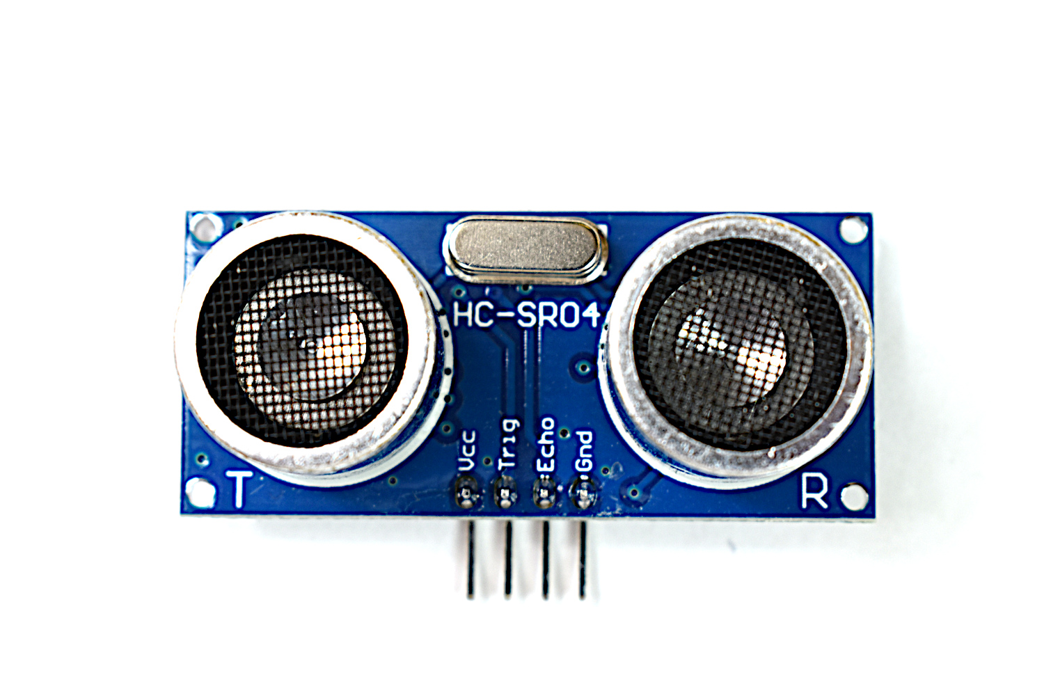
Ultrasonic distance sensor that is capable of measuring distances from 2cm - 4m. The HC-SR04 can be used in obstacle detection, radar emulators, and projects involving mapping of areas.
Included in the HC-SR04 Package:
1x HC-SR04 Sensor
Features of the HC-SR04:
5V Operating Voltage
15mA Peak Current Consumption
40Hz Sample Rate
Valid Detection Range: 2cm - 4m
40 kHz Ultrasonic Pulse
Compatible with Arduino, Raspberry Pi
A typical healthy human is capable of distinguishing a range of frequencies between 20Hz and 20kHz. Frequencies above this range, called ultrasound, are inaudible to humans because of physical and neural limitations set by our auditory systems. Sound, much like light, is a great scientific tool because of its predictable behavior and manipulative properties. The primary applications of ultrasound are in civil and biomedical engineering. Ultrasound is remarkably tunable and is often used for non-destructive testing and surgical applications. Here, the application is time-of-flight calculation and the method is straightforward. Ultrasound can be treated as a disturbance traveling through a medium (air). As such, we can define the linear relationship between distance, velocity, and time as:

where c is the speed of sound, d is distance, and t is time. The trick to ultrasonic distance calculation comes in the geometry setup and the time delay between the transmitted and received pulses:

Here we define Δt as the time it takes for a series of transmitted pulses to be emitted, incident on an object some distance away, and return back to the location of transmission. This is the basis for ultrasonic, and any linear, time-of-flight calculation.
HC-SR04 Sensor and Arduino
Focus will now shift from physics to instrumentation. The ultrasonic distance sensor, HC-SR04 (and its many variations), is common in maker electronics because of its simple and intuitive design. The sensor sends out a series of 40kHz pulses and listens for a return signal. The Arduino can be programmed to calculate the time difference between pulse transmission and reception to approximate the distance of an object. A typical wiring diagram for the HC-SR04 is shown below, with one caveat being that the SIG of the diagram below would be Trig and Echo on HC-SR04. The Trig should be connected to digital pin 2 on the Arduino Uno and the Echo should be connected to pin 3.
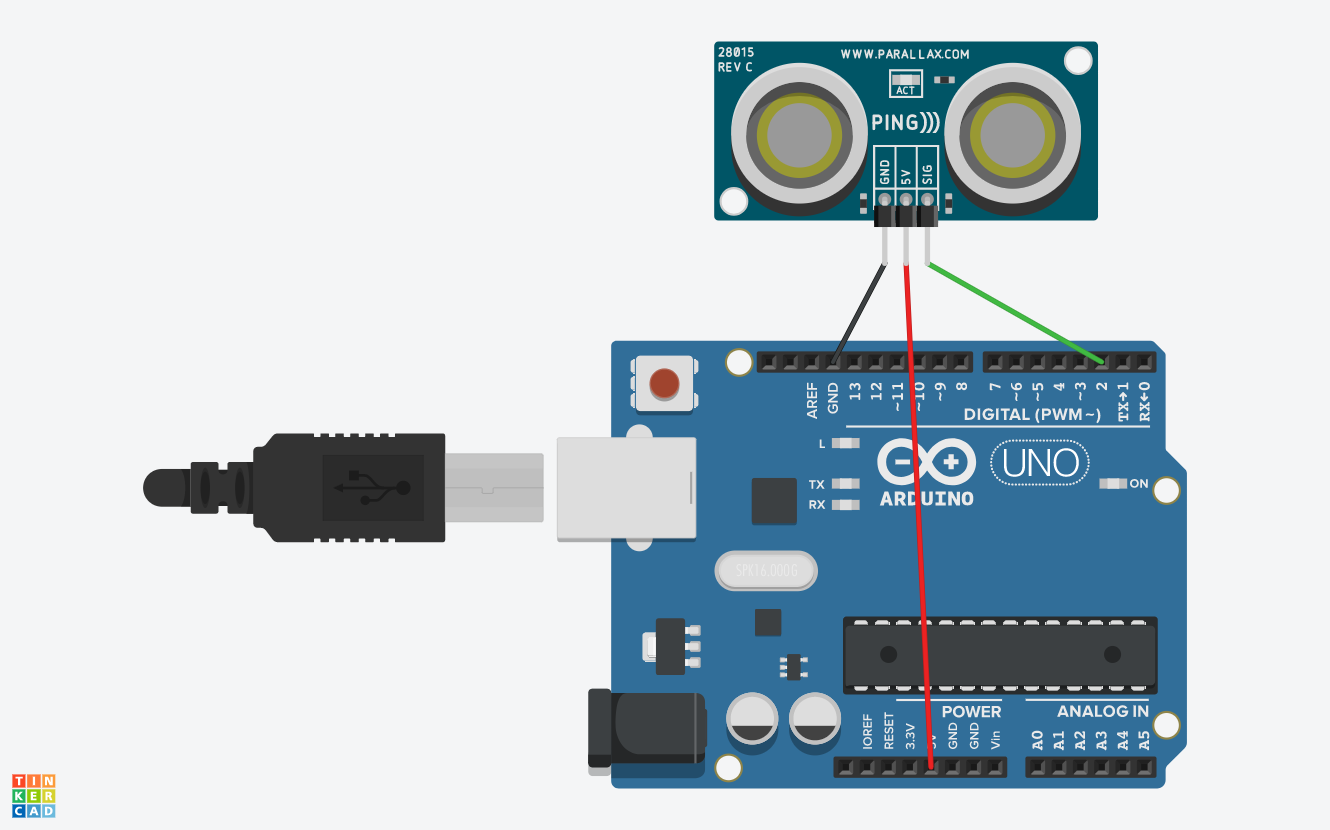
Wiring diagram for ultrasonic sensor. Note that the SIG output shown here should be Trig and Echo, connected to pins 2 and 3, respectively.
Below is the basic implementation of the ultrasonic time-of-flight calculation using the Arduino IDE.
At this point, your Arduino board should be spitting out reasonable estimates of an object some distance away from the sensor. If there are any issues, it is likely a programming error or wiring issue. Otherwise, if your values are reasonable and you are satisfied with your results, then you are finished with this tutorial. However, if you are seeing an error in your measurements, then please continue reading as I discuss calibration and how to correct the HC-SR04 for drift or factory inaccuracies.
Calibrating The HC-SR04 For More Accurate Readings
Video showing how to after-market calibrate a HC-SR04 ultrasonic distance sensor.
The sensor used for my experiments was exhibiting consistent error when measured over several distances. The error was small, but noticeable and consistent enough that I decided to investigate its calibration. I used grids of engineering paper and a moving target to record several time-of-flight (TOF) distance calculations to determine how well the sensor was approximating the target's location. I recorded several TOF measurements using Python's serial read function. This made plotting and understanding the behavior conclusive. The raw data from the moving target experiment is shown below:

Plot showing the raw moving target experiment. Each horizontal trend signifies a 1 inch move away from the sensor.
It is not clear from the plot above, however, after inspection and conversion to distance it is clear that the sensor had some drift to the true values. Consequently, I decided to use Python's polyfit tool (in numpy) and attempt to find a trend in imprecise data. The basic idea behind implementation of polynomial regression is that sensors often drift over time and under certain circumstances (temperature/humidity changes, component stress from usage over time, physical stress, etc.), so it is not uncommon for sensors to need calibration from time to time. I used a first order regression to model a linear drift and used the data gathered from the moving target readings against the real, measured distances and found the following constants:

The d in the above equation signifies the calculated distance using the traditional TOF physical model. After finding those constants for the linear model and using the linear model to adjust the original calculated values, the error was minimized and the produced the following results:

The improvement on the original estimates is huge. Upon substitution back into the original Arduino code, the errors are completely minimized. Now, the values printed on the Arduino serial monitor are completely accurate and within a reasonable margin of error. The HC-SR04 sensor is reliable and fully functional (I tested mine up to 7 ft), and the error was less than 1% (beyond 1ft) and less than 10% (less than 3 inches). It proves, once again, that the science is backed by nature, but instrumentation needs to be backed by humans.
Final Relevant Codes
# Plotting the Results from HC-SR04 Calibration
#
#
import matplotlib.pyplot as plt
import csv, math
import numpy as np

dat_vec = [1.05,1.79,2.73,3.57,4.4,5.48,6.27,10.7,20.5,30.8,41,51.2,61.45,82.1] # these are values that the typical time-of-flight algorithm spits out, uncorrected

x_poly = [1,2,3,4,5,6,7,12,24,36,48,60,72,96] # these are the expected values (measured with precision)

order_num = 1 # order of polynomial fit [linear = 1]

plt.figure(figsize=(12,9))
poly_fit = np.polyfit(dat_vec,x_poly,order_num) # fit the data to the measured values

print(poly_fit) # print them to plug them back into Arduino code

# Plot, if desired

p = np.poly1d(poly_fit)
plt.plot(dat_vec,x_poly,linewidth=4,label='Exact',color='#3a2a29')
plt.plot(dat_vec,p(dat_vec),linestyle='--',color='#b39a7c',label='Corrected',linewidth=4)

plt.plot(dat_vec,dat_vec,linestyle='-',label='Uncorrected',color='#7e8f7c',linewidth=4)

ax = plt.subplot(111)
ax.spines["top"].set_visible(False)
ax.spines["right"].set_visible(False)

ax.get_xaxis().tick_bottom()
ax.get_yaxis().tick_left()

plt.title("Calibration Correction for HC-SR04 Ultrasonic Sensor",fontsize=22)
plt.ylabel("Expected Distance [inches]",fontsize=20)
plt.xlabel("Recorded Distance [inches]",fontsize=20)

plt.legend(loc=2)
plt.savefig('data_hc_sr04_fitting.png',transparent=True)