The MPU9250 is a 9 degree-of-freedom (9-DoF) inertial measurement unit (IMU) that houses an accelerometer/gyroscope combination sensor (MPU6050) and a magnetometer sensor (AK8963). The data read by the accel/gyro (MPU6050) and mag (AK8963) can be best understood by first investigating the configuration of each sensor’s coordinate system. Below is the coordinate composition for both sensors:

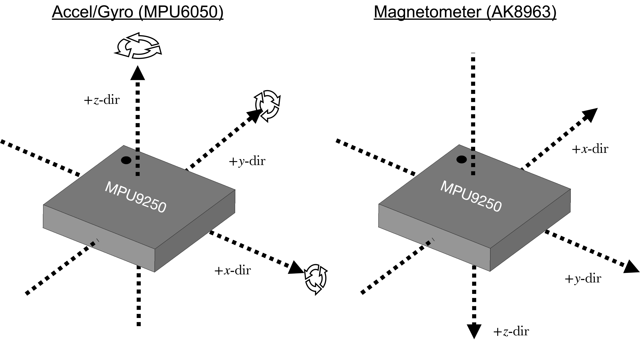
The accelerometer coordinate system uses a somewhat traditional cartesian coordinate system. Similarly, the gyroscope uses a counter-clockwise rotation as the positive rotation direction. The magnetometer switches the x- and y-directions, while reversing the direction of the z-direction amplitude. These conventions will come into play during calibration and will be clarified and discussed for each of the three sensors.

The coordinate references will be essential for understanding the data being read by the MPU9250 and developing methods for calibrating the IMU.

Range of each Sensor:

• Accelerometer - will be calibrated under the range of 0g-2g

• Gyroscope - will be calibrated under the range of 0dps - 250dps

• Magnetometer - will be calibrated under the range of 0μT - 4800μT

The MPU9250 will be attached to our Calibration Block which will allow for rotation along each axis and ensure that the sensors are calibrated for best alignment with gravity (accelerometer) and rotation about each axis (magnetometer).

The simplest calibration of an IMU consists of calculating the offset for each axis of the gyroscope. The gyroscope is the easiest calibration due to the expected readings outputted under steady conditions. Each of the three axes of the gyro should read 0 degrees-per-second (dps, °/s) when the IMU is not moving. The offsets can be measured by first taking some readings while the IMU is not moving, then using those values as ‘offsets’ when reading the gyro values in the future. This is merely the simplest calibration method for the IMU and suffices for most casual uses of the gyroscope and IMU. There are a range of higher-order gyroscope calibration routines, which can be found at the following links (with application descriptions):

• “In-use calibration of body-mounted gyroscopes for applications in gait analysis” by Sergio Scapellato et al. (2005)

• “A Novel Tri-Axial MEMS Gyroscope Calibration Method over a Full Temperature Range” by Haotian Yang et al. (2018)

• “Improved multi-position calibration for inertial measurement units” by Hongliang Zhang (2009)

• “An Algorithm for the In-Field Calibration of a MEMS IMU” by Umar Qureshi and Farid Golnaraghi (2017)

The MPU6050’s gyroscope offsets can be found by recording a sample chunk of data from each axis and using the average of each sample. The gyro calibration routine (and all other codes used in this tutorial) can be found at this project’s GitHub page:

The gyroscope offset calculation sample code is also given below:

The output from the code above plots the triple-axis gyroscope for both uncalibrated and calibrated values for a number of samples prescribed in the variable “cal_size” (chosen as 500 samples in our case). The example output for our gyroscope is shown below:

It is easy to see that the offsets are essential for minimizing the expected minimal values under steady IMU conditions.

We can further test the calibration of the gyroscope by integrating an array of angular velocity values over time under a known rotation. For example, we can rotate the IMU Calibration Block by 180° and integrate the gyro over time to verify that the gyroscope is functioning properly.

By integrating the gyroscope’s angular velocity, approximations of angular displacement can be made:

For discrete points, a numerical integration technique is required, for which we use trapezoidal numerical integration:

The ‘scipy’ package in Python has a great implementation of the trapezoidal numerical integration, which makes it easy to approximate rotation of the IMU by integration of the gyroscope. An example implementation of the gyroscope integration is given below in the plot:

The gyroscope approximates the 180° rotation to be roughly 179.8°, which is quite accurate. It also tells us that the directionality of the IMU is accurate, as in the case above the rotation was carried out in the counter-clockwise direction. Thus, we have a reasonably accurate calibration of the gyroscope on the MPU9250 (MPU6050). Of course, the validation above is for a very steady and idealized rotation. Nonetheless, the gyro can be considered as zeroth-order calibrated. In the next section, the accelerometer will be calibrated similarly, but with a first-order approximation, which is slightly more involved and requires three calibration steps for each axis. The accelerometer will also be validated by numerical integration in a similar manner as the gyroscope.

Calibration of the accelerometer requires taking advantage of the acceleration due to gravity, which we can use in the positive and negative orientation of the IMU. Additionally, we can also position the IMU perpendicular to gravity in order to acquire a third calibration point. This results in three unique values that can be combined to formulate a linear fit between the three values and the values outputted by each axis of the accelerometer.

The calibration procedure for the accelerometer is as follows (for each axis):

These three calibrations should be done for each of the 3-axes. The three points will allow for least-squares fitting of a first-order model to the scale factor and offset (slope and intercept) of each axis of the accelerometer.

The Python code used to calibrate the accelerometer is given below:

The code above takes the user through the calibration steps for each of the three axes and outputs a plot similar to the following:

The above calibration represents the IMU attached to the Calibration Block with the z-direction pointed upward. This is why we see an acceleration of 1g in the z-direction, and near zero values in the other two directions.

We can again see the benefit of the calibration for each axis in terms of the linear fit below:

Next, validation of the accelerometer will be carried out by moving the IMU Calibration Block a known distance in a chosen direction. The corresponding acceleration measured by the accelerometer will be integrated twice to approximate displacement.

The accelerometer calibration can be validated in a similar manner as the gyroscope - by numerical integration. The difference between the gyroscope integration and the accelerometer integration is that the acceleration values will be integrated twice to output an approximate displacement of the IMU, according to the following integration:

Again, the above relationship needs to be discretized in order to make it suitable for real-world movements, which first requires integration of acceleration to first approximate velocity:

Next, the velocity array must be integrated to then approximate displacement:

In Python, we first use ‘intergrate.cumtrapz’ which implements trapezoidal numerical integration in step-by-step increments. The first integration gives a velocity vector, while the second integration results in a displacement array.

The double integration of the acceleration test makes several assumptions:

1. The object (IMU Calibration Block) is at rest

2. The time between samples is known (likely not uniform for the IMU)

3. The IMU is sliding in one direction

4. The acceleration axis is perpendicular to gravity (0g influence of gravity)

Under these assumptions, the accelerometer values can be easily integrated in one direction. Below is a demonstration of the IMU Calibration Block being slid across a tap measure in one direction. The measured displacement will be compared with the twice-integrated accelerometer data for validation of the accelerometer calibration.

The code given below either calibrates the accelerometer or takes calibration coefficients as input (from a previous calibration). It then employs a 4th-Order Butterworth digital filter to smooth the signal, and ultimately outputs acceleration, velocity, and displacement to depict the integration results:

An example output is also given below, for a test case of the IMU sliding in the +y-direction for 0.5m:

Several observations can be made for the plot above:

• The acceleration is not zero, even after calibration (likely due to an unbalanced table)

• The acceleration starts positive (acceleration), crosses zero, then goes negative (deceleration)

• The velocity is positive throughout (forward movement)

• The displacement is positive (forward movement)

• The velocity and displacement are constantly changing due to the imbalanced acceleration (unbalanced table)

The approximation of displacement was found to be roughly 0.4m for the 0.5m test. This inaccuracy is due to the double integration and uncertainty associated with the sensors, along with the imperfect calibration. This can be remedied by ensuring the IMU is perpendicular to gravity during calibration (with a level) and also ensuring the test is being done on a level surface.

In this tutorial, calibration of the gyroscope and accelerometer on the MPU9250 (MPU6050) was explored through various methods. The gyroscope was calibrated under steady conditions by calculating the mean offset from a measurement sample array. The accuracy of the gyroscope was explored by first integrating the angular velocity over time and looking at the result after a known rotation. The accuracy after 180 degrees of rotation was found to be less than 1-degree, which is quite accurate. This is, of course, under very idealized conditions: smooth and small angle rotation. Similarly, the accelerometer was tested for a range of three calibration points: +1g, -1g, and 0g. These three points were fitted to line using least-squares methods. The accelerometer was also integrated, this time twice, to approximate the movement of the IMU over a known displacement. The accuracy of this method was found to be quite error prone, likely due to the following factors: the IMU was placed on a table not perfectly perpendicular to gravity, the double integration results in greater errors. The accelerometer was also filtered to smooth the signal (which was quite noisy, particularly when sliding on a table). The filtering can also be done on the gyroscope. In Part III, the next and final entry of this series, the magnetometer will be calibrated. The magnetometer is much more involved than both the gyro and accelerometer calibration due to the requirement of two axis components for calibrating under Earth’s magnetic field. An ensemble calibration will also be introduced with a routine to save all calibration coefficients for all three sensors (for all 9-DoF). This will allow for users to calibrate once and employ the calibration coefficients into their application.

See More in Raspberry Pi and Engineering: