Arduino Pitot Tube Wind Speed and Airspeed Indicator - Theory and Experiments
Named after its french creator, Henri Pitot, the pitot tube is a device used to approximate the speed of vehicles traveling by air and water. An in-depth article on NASA's website is dedicated to pitot tubes (also called pitot-static tubes, Prandtl tubes), where it cites the primary application as airspeed indicator on aircraft. For more information on design and limitations of the instrument, I recommend perusing that page. For this tutorial, only the basic theory is explored using Bernoulli's equation and a practical application. An inexpensive pitot tube and a digital differential pressure sensor are used to measure pressure, which is converted to a digital signal using an Arduino board.
Pitot Tube in the foreground and the velocity plot in the background
For fluid mechanics problems involving incompressible, frictionless flow; Bernoulli’s principle is a valid place to start. Bernoulli’s principle can be written as a pressure balance between two sections:
where ρ, v, P, h are the fluid density, velocity, pressure, and height of the flow section, respectively. The subscripts a,b represent two differing sections of the flow section. In our case, we need the stagnation pressure, which is the pressure due to the static pressure and the pressure incident on the bend in the pitot tube. A setup of this can be seen below:

Assuming no change due to gravity and no velocity at the stagnation point, we can see how the pitot tube can measure both velocity and static pressure:
Additionally, we have a separate section that allows only static pressure to be measured via ports perpendicular to the flow direction (static ports). We can now measure the stagnation pressure and the static pressure separately:
subtracting the two:
and if we solve for velocity as a function of the pressure differential:
This experiment consists of a pitot tube and pressure differential sensor combination and an Arduino board. The method of testing the pitot tube is up to the user - for example, I will be using a small DC fan and a 0.5 inch tube to measure the efficiency of the fan. However, the user may want to measure a different parameter such as: drone airspeed, wind speed, or car velocity. Below is a list of parts both necessary and particular to this experiment:
Pitot Tube and MLXV7002DP - $32.99 [Amazon] or $48.89 [Amazon]
NOTE: these appear to be unavailable at the moment, but users can buy a similar differential pressure sensor and pitot tube from our store: Pitot Tube Airspeed Sensor for Arduino and Raspberry Pi - $45.00 [Our Store]
Arduino Uno - $13.00 [Our Store]
5V DC Fan - $7.98 (4 pcs) [Amazon]
0.5 inch Tubing - $12.39 (10 ft.) [Amazon]
Jumper Wires (male-to-male) - $0.45 (3pcs) [Our Store]
Breadboard - $3.00 [Our Store]

Named after its french creator, Henri Pitot, a pitot tube is a device used to approximate the speed of vehicles traveling through air and other fluids. Pitot tubes, also called pitot-static tubes and Prandtl tubes, are primarily used as airspeed indicators on drones, airplanes, and other rotorcraft. Pitot tubes use basic fluid dynamics and the Bernoulli equation to approximate airspeed, or relative velocity, of a moving vehicle/flying object. The pitot tube here can be combined with our XGMP3v3 Differential Pressure Sensor to measure pressure, which is then converted to a digital signal using an Arduino board or other analog-to-digital converter (ADC). This final differential pressure can be used to derive airspeed or velocity of a moving object.
Included in the Pitot Tube Airspeed Sensor Package:
1x Metal Pitot Tube
2x Acrylic 2.5mm ID Tubing (75cm in Length)
1x XGMP3v3 Differential Pressure Sensor
1x JST-XH 3-Wire Connector (Colors May Vary)
Features of the Pitot Tube Airspeed Sensor:
3.3V Supply Voltage
0.2V - 2.7V Analog Output
Dimensions (Pitot Tube): 100mm x 16mm x 6mm
Flexible 2.5mm Tubing (75cm Length)
Aluminum Machined Metal
Selectable Pressure (Velocity) Range:
-0.5kPa to +0.5kPa -> -28m/s to +28m/s
-1.0kPa to +1.0kPa -> —41m/s to +41m/s
-2.5kPa to +2.5kPa -> -64m/s to +64m/s
Features of the XGMP3v3 Differential Pressure Sensor:
3.3V Operating Voltage
24mA Max Power Consumption (10mW)
Analog Output Range: 0.2V - 2.7V
Measurement Accuracy: ±2.5% Full-Scale [kPa]
Temperature Compensated from 0°C - 60°C
Selectable Pressure Span:
-0.5kPa to +0.5kPa (Most Sensitive)
-1.0kPa to +1.0kPa
-2.5kPa to +2.5kPa (Similar to MPXV7002DP)
Absolute Maximums: ±2x Pressure Max, -10°C to 85°C Operating Temperature
For Use with Non-Corrosive Gas (Air, Inert [Helium, Neon, Argon, etc.])
JST-XH Connector Makes Connection to Raspberry Pi or Arduino Simple
The wiring for the Arduino and pressure sensor is simple: we wire the analog output from the MPXV7002DP sensor to one of the analog inputs on the Arduino board.
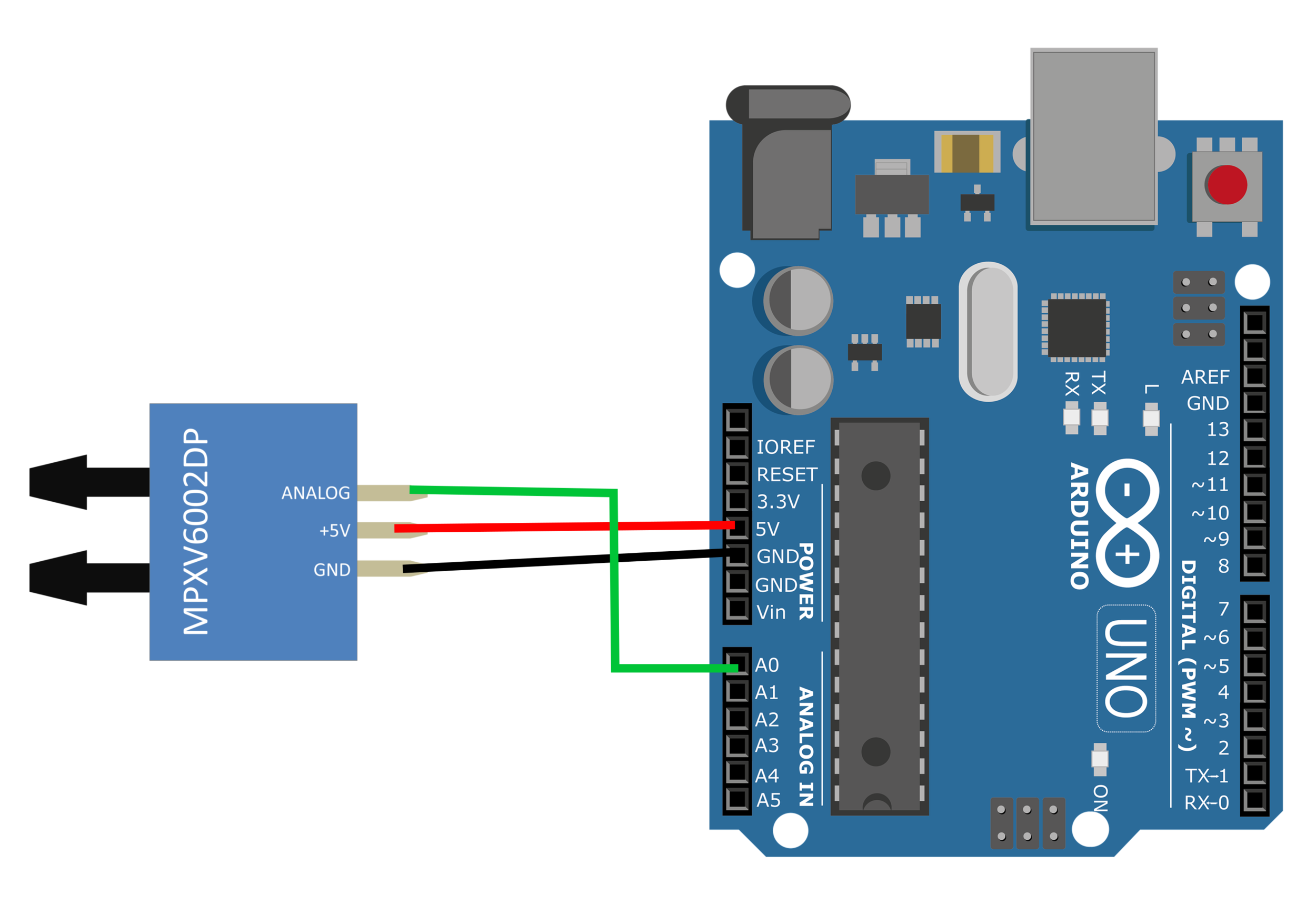
MPXV7002DP Wiring for Differential Pressure Measurement
Since the MPXV7002DP handles the pressure differential calculation and the pitot tube handles the pressure measurement of both stagnation pressure and static pressure - a lot of the work to be done is in the calculation of velocity, not in the electrical wiring. Therefore, the electronics portion of this tutorial is quite simple. In the next and following sections, the conversion from voltage reading to pressure differential, and subsequently to velocity is covered.
The MPXV7002DP is a sensor that relates the pressure differential between its two inputs. In the datasheet, the manufacturer provides the calibration relationship between the output voltage and pressure difference. This plot is shown below:

Voltage vs. Pressure relationship for representing the pressure differential as a function of voltage. This plot will be essential for relating the voltage read by the Arduino analog pin back to the pressure differential between the stagnation pressure and static pressure.
A few notes on the plot above:
- The bounds on pressure don't change despite the supply voltage - meaning we can use either 3.3V or 5.0V
- The pressure maximum and minimum put the velocity limits around 65 m/s
- The raw Arduino 5.0V supply is quite noisy, which results in high error
Since the transfer function is not quite right, I will use a point-slope method to re-derive the transfer function and then re-plot below. To start, we use the linear slope equation:
where m, b are the slope and y-intercept of the line, respectively. And y is the voltage reading, and x is the pressure difference between the input pressures (stagnation pressure and static pressure in our case). By selecting two points on the line above, we can solve for m and b:
which can be written in equation form as:
This is the relation for converting pressure to voltage, and if we solve for x , we can get the equation for going from voltage to pressure:
MPXV7002DP Conversion Table
| Pressure [kPa] to Voltage [Volts] | Voltage [Volts] to Pressure [Pa] |
|---|---|
The table above is a summary ofthe conversion between pressure and voltage and vice-versa. Above, Vr is the voltage reading from the Arduino, and Vs is the supply voltage (Arduino either 3.3V or 5.0V - or some other external supply below 5.0V). The pressure, P, is in either kPa or Pa depending on the conversion direction. When going from pressure to voltage, we want to use kPa to match the plot units. When going from voltage to pressure, we convert to Pa so that we can match the units of the pitot tube equation.
NOTE: when converting from voltage to pressure, be sure to multiple by 1000 to go from the units of the pressure differential (kilopascal) to S.I. units (Pascals).
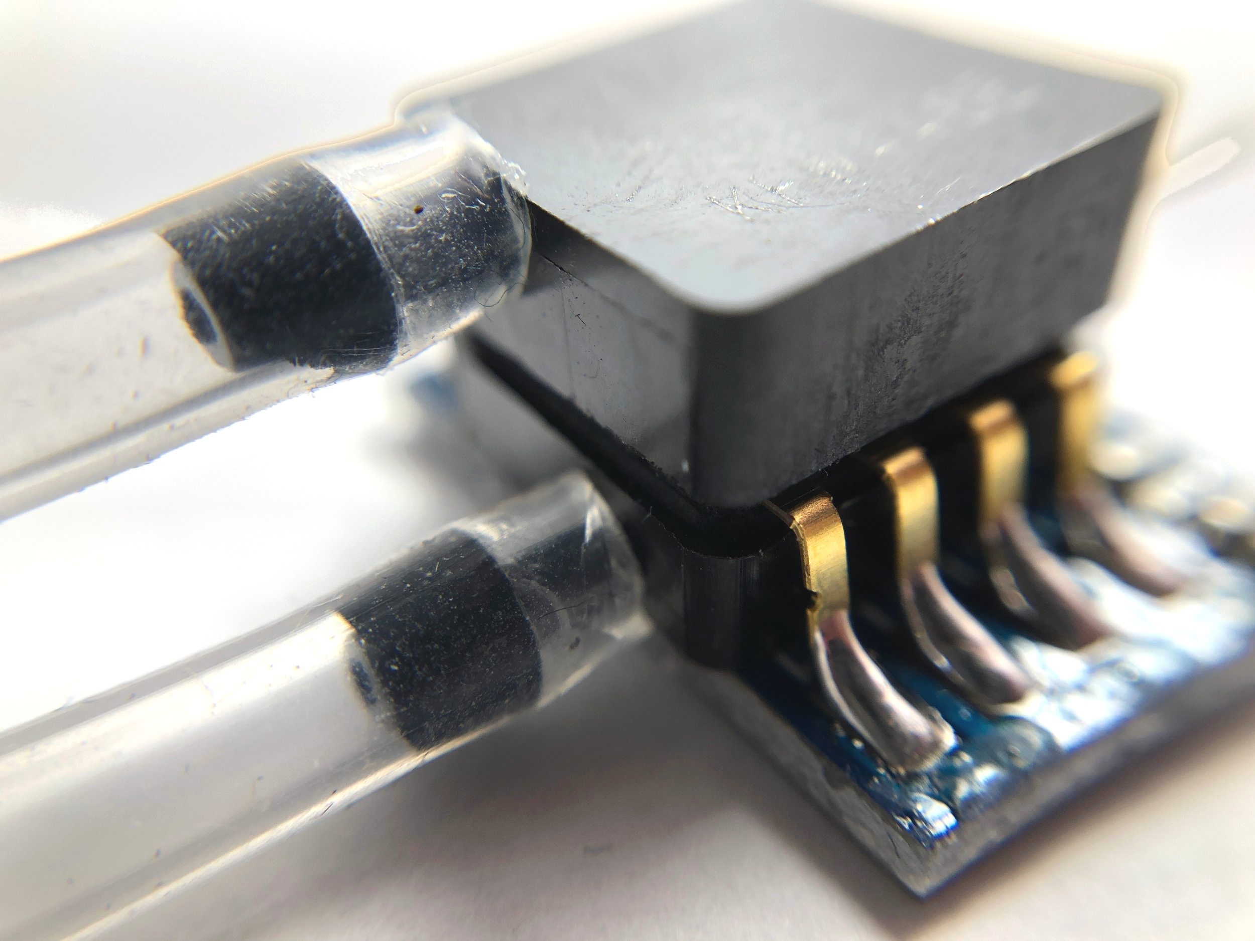
At this stage, the user must connect their pitot tube to the pressure differential sensor. Be sure that the tubes are not bend or pinched in any area, otherwise results may be misleading due to friction or turbulence. Below is a drawing of the pitot tube connected to the MPXV7002DP, which is subsequently wired to the Arduino board:

Wiring the pitot tube to the MPXV7002DP sensor, which is wired to the Arduino uno board.
Now in order to properly approximate velocity, we need to relate the pitot tube velocity equation to the pressure differential read as a voltage by the MPXV7002DP sensor. We can do this by citing the velocity equation:
and the pressure differential from the voltage readout:
and recognizing that ΔP = Pstagnation − Pstatic , we can make the following relation between our input parameters, our voltage readout, and the resulting velocity approximated by the pitot tube:
One final note: don’t forget the conversion from bits to voltage:
Finally, one unified equation for converting from ADC values to velocity can be written as:
where R is the reading from the Arduino analog pin, ρ is the density of the fluid (air in this case), and (210-1) is the 10-bit resolution of the Arduino's ADC (there's a -1 because we include 0).
Once the pitot tube and MPXV7002DP are connected and wired to the Arduino board, the user should take some basic analog readings to test the system and its response. You can do this by blowing into the pitot tube or using a fan. The first thing to note is the baseline value. It should be 1023/2 = 511.5, however, this value is not an integer - so we can blindly assume either 511 or 512 are the expected baseline values. Now, in my case, the baseline was a bit higher (534), so I implemented an offset average in the setup portion of the Arduino code. This also means that when starting up the Arduino, there should be no flow such that the code can configure the baseline.
The full Arduino code is shown below, also with an averaging loop which is meant to stabilize the output value (though there is still a lot of noise in the velocity measurements):
//Routine for calculating the velocity from
//a pitot tube and MPXV7002DP pressure differential sensor

float V_0 = 5.0; // supply voltage to the pressure sensor
float rho = 1.204; // density of air

// parameters for averaging and offset
int offset = 0;
int offset_size = 10;
int veloc_mean_size = 20;
int zero_span = 2;

// setup and calculate offset
void setup() {
  Serial.begin(9600);
  for (int ii=0;ii<offset_size;ii++){
    offset += analogRead(A0)-(1023/2);
  }
  offset /= offset_size;
}

void loop() {
  float adc_avg = 0; float veloc = 0.0;

// average a few ADC readings for stability
  for (int ii=0;ii<veloc_mean_size;ii++){
    adc_avg+= analogRead(A0)-offset;
  }
  adc_avg/=veloc_mean_size;

  // make sure if the ADC reads below 512, then we equate it to a negative velocity
  if (adc_avg>512-zero_span and adc_avg<512+zero_span){
  } else{
    if (adc_avg<512){
      veloc = -sqrt((-10000.0*((adc_avg/1023.0)-0.5))/rho);
    } else{
      veloc = sqrt((10000.0*((adc_avg/1023.0)-0.5))/rho);
    }
  }
  Serial.println(veloc); // print velocity
  delay(10); // delay for stability
}
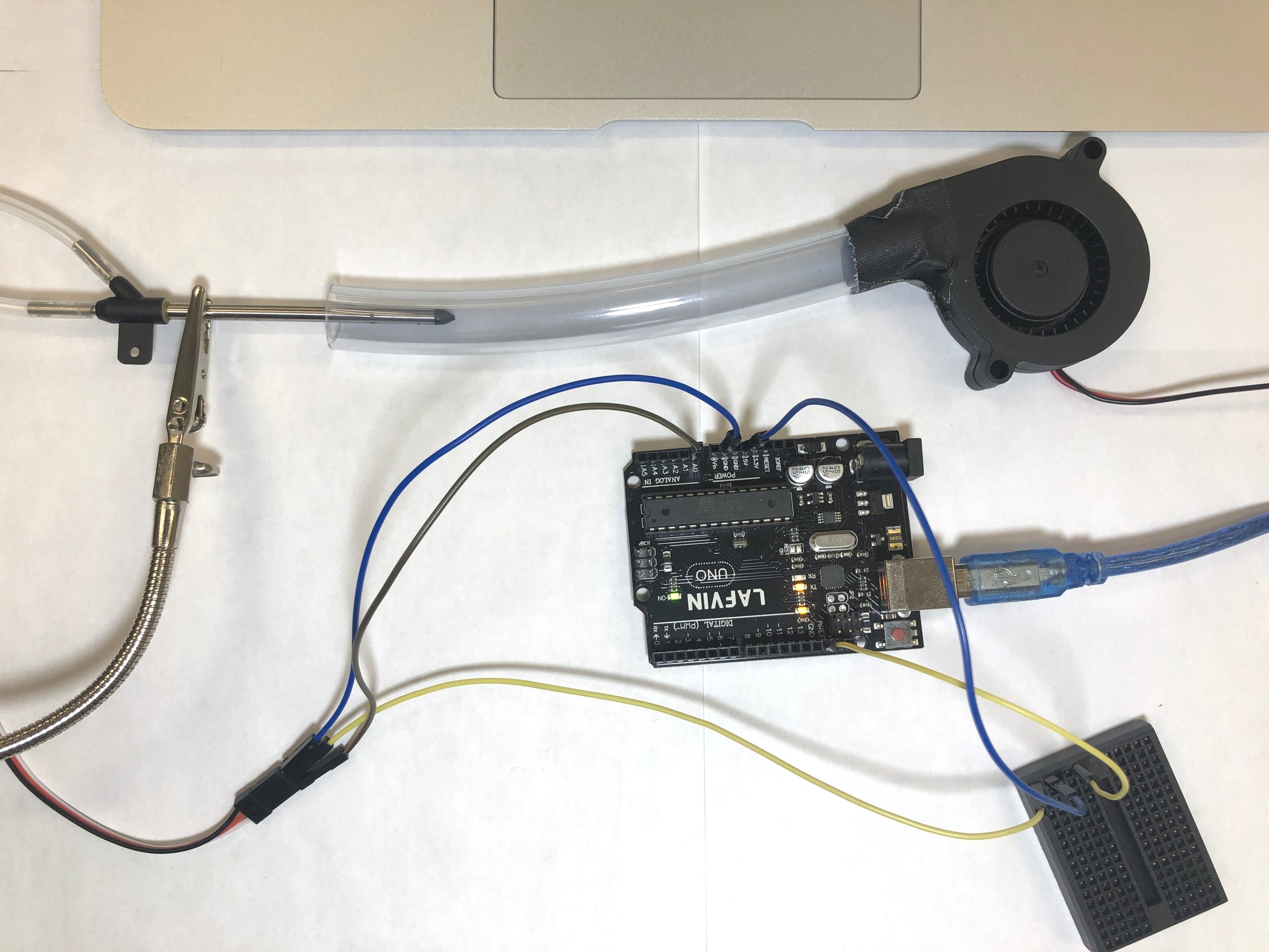
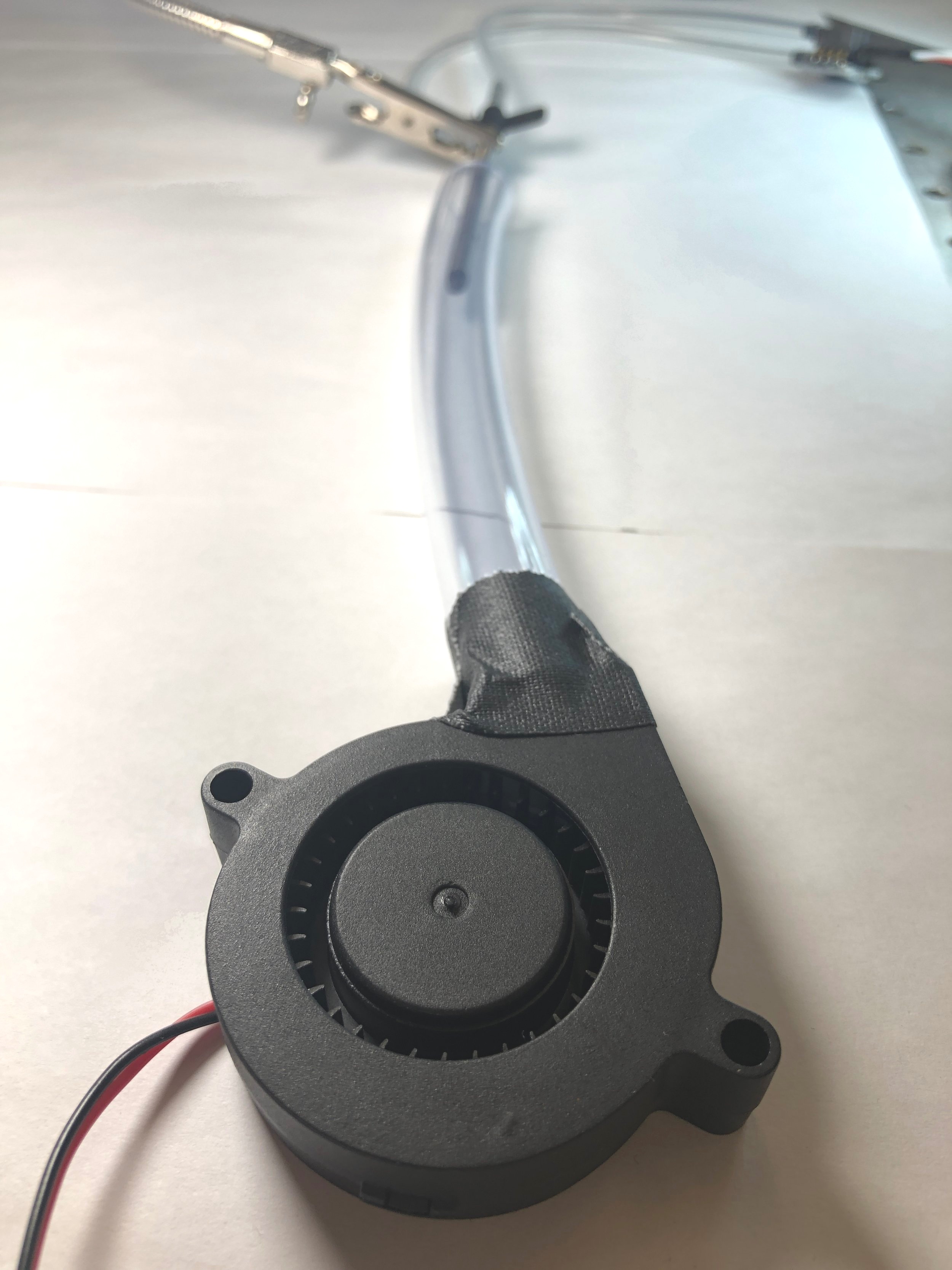
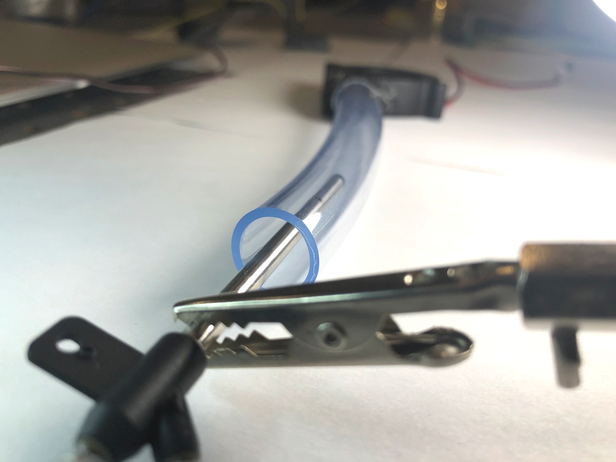
As stated earlier, this experiment uses a 0.5 inch cylindrical pipe and a 5V blower fan (which I ran at 12V) to analyze the volumetric flow rate through the pipe using a pitot tube. This will allow us to both test the pitot tube and quantify the efficiency of a cooling fan. Below is a series of photos of the setup:
Below is a video of the pitot tube measuring velocity in real-time. The pitot tube measures the velocity around 14.5 m/s within the tube.
Now that we know the velocity within the tube, we calculate the volumetric flow rate of the fan and compare it to the manufacturer’s value. To start, we can assume that the velocity is uniform due to the shortness of the pipe, which means the velocity profile hasn’t developed in the tube (in the presence of friction). So we measured the velocity at the center of the tube and can invoke conservation of energy:
as stated before, the inner diameter of the acrylic pipe is 0.5 in. (0.0127 m) so we can quantify the volumetric flow rate:
and previously we found the velocity in the tube to be about 14.5 m/s
And to compare with the manufacturer’s value, we convert to CFM (cubic feet per minute):
This leads to our actual volumetric flow rate:
Q ≈ 3.9 CFM
and this is quite a satisfying result, because the manufacturer cites the maximum flow rate as 5 CFM, which is not too far off. Not to mention the fact that the areas between the outlet of the fan and the pipe aren’t identical, the tube is slightly bent, and our measurements are quite noisy.
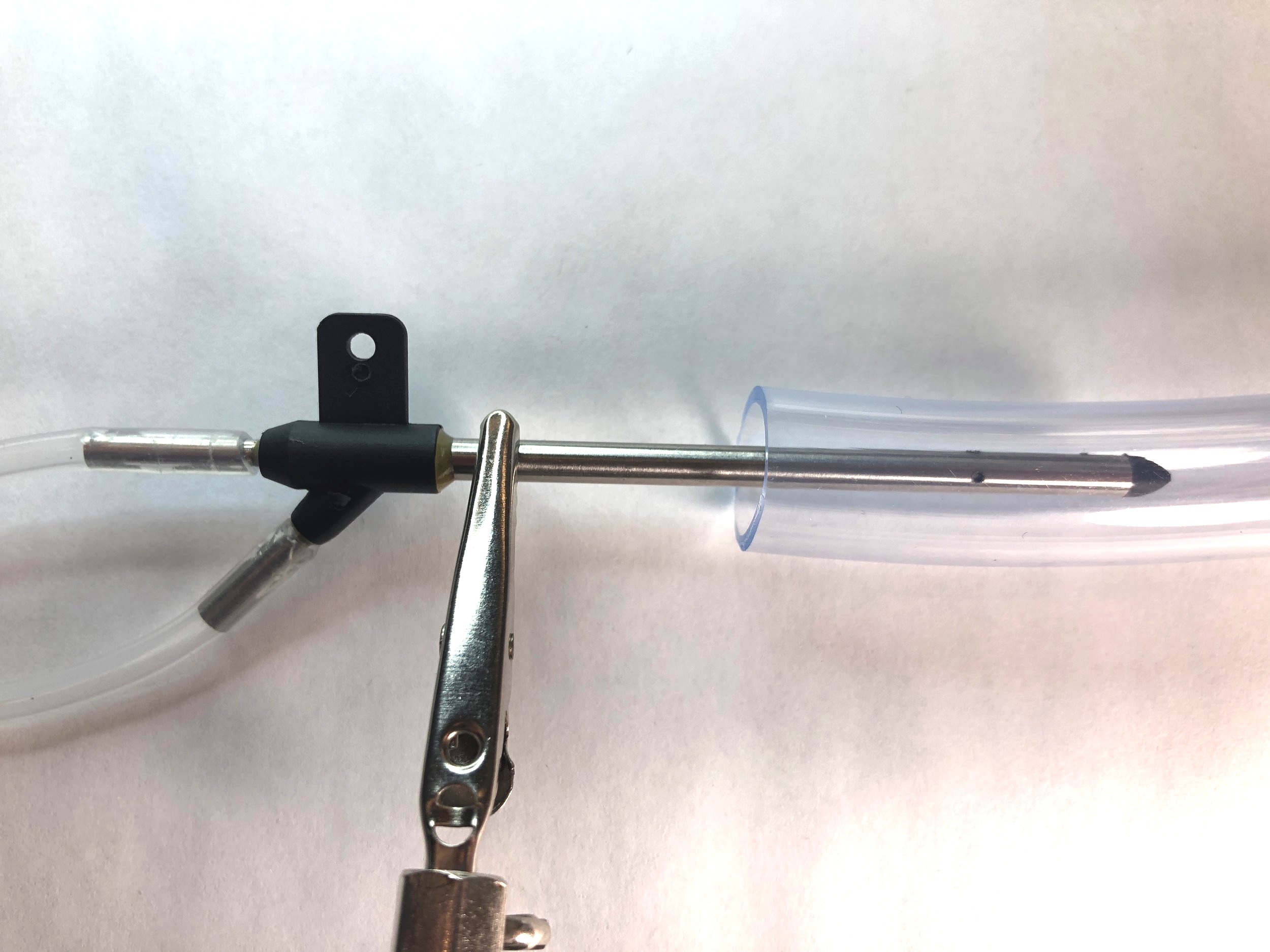
Tip of pitot tube used in this experiment
The pitot tube is an instrument widely used to measure the speed of a flowing fluid. I started the tutorial by deriving the pitot tube velocity approximation from Bernoulli’s principle. I also introduced the conversion from voltage to pressure differential from the MPXV7002DP sensor, and the subsequent conversion from pressure differential to flow velocity. Lastly, I used the pitot tube to measure the volumetric flow rate of a DC fan. The result was about 80% of the manufacturer’s cited efficiency (we measured 15.6 CFM, the datasheet cites 20 CFM). This tutorial was meant to introduce the user to the pitot tube by using a real-world example, while also exploring a classic engineering experiment that utilizes classic fluid mechanics techniques for solving problems.
See More in Engineering: